
Regression - Mechanics and Interpretation
Housecleaning
- Assignment 5 review
- All project instructions moved to project page under assignments tab
Objectives
- You can fit a regression with
statsmodelsorsklearn - You can view the results visually or numerically of your model with either
- You can interpret the mechanical meaning of the coefficients in a regression
- continuous variables
- categorical a.k.a qualitative variables with two values (aka "dummy" or "binary" variables)
- categorical a.k.a qualitative variables with more than values (aka "fixed effects")
- how an interaction term changes interpretation
- You understand what a t-stat / p-value does and does not tell you
- You can measure the goodness of fit on a regression
- You are aware of common regression analysis pitfalls and disasters

Regression
Basics and notation
- Regression is the single most important tool at the econometrician's disposal
- Regression analysis is concerned with the description and evaluation of the relationship between a variable typically called the dependent variable, and one or more other variables, typically called the independent or explanatory variables.
- Alternative vocabulary:
| y | x |
|---|---|
| dependent variable | independent variables |
| regressand | regressors |
| effect variable | causal variables |
| explained variable | explanatory variables |
| features |
The regression "model" and terminology
If you want to describe the data (the scatterplot below, e.g.) you might fit a straight line
\begin{align} y=a+\beta x \end{align}But that line can't exactly fit all the points of data (it's impossible to find all determinants of $y$ and $y$ may be mismeasured), so you need to account for the discrepancies, and so we add a "error term" or "disturbance" denoted by $u$
\begin{align} y=a+\beta x+u \end{align}Now, we want to estimate $a$ and $\beta$ to best "fit" the data. Imagine you pick/estimate $\hat{a}$ and $\hat{\beta}$ to fit the data. If you apply that to all the X data points like $\hat{a} + \hat{\beta}x$ , then you get a predicted value for $y$:
\begin{align} \hat{y} = \hat{a} + \hat{\beta}x \end{align}We call $\hat{y}$ the "fitted values" or the "predicted values" of y. And the difference between each actual $y$ and the predicted $\hat{y}$ is called the residual or error:
\begin{align} y-\hat{y} = \hat{u} = \text{"residual" aka "error"} \end{align}The goal of estimation (any estimation, including regression) is to make these errors as "small" as possible. Regression is aka'ed as "Ordinary Least Squares" which as it sounds, takes those errors, squares them, adds those up, and minimizes the sum
\begin{align} \min & \sum(y-\hat{y})^2 = \min & \sum(y-\hat{a} + \hat{\beta}x) \end{align}So, to combine this with the "Modeling Intro" lecture, regression follows the same steps as any estimation:
- Select a model. _In a regression, the model is a line (if you only have 1 X variable) or a hyperplane (if you have many X variables).)
- Select a loss function. In a regression, it's the sum of squared errors.
- Minimize the loss. You can solve for the minimum analytically (take the derivative, ...) or numerically (gradient descent). Our python packages below handle this for you.

# load some data to practice regressions
import seaborn as sns
import numpy as np
diamonds = sns.load_dataset('diamonds')

# this alteration is not strictly necessary to practice a regression
# but we use this in livecoding
diamonds2 = (diamonds.query('carat < 2.5')               # censor/remove outliers
            .assign(lprice = np.log(diamonds['price']))  # log transform price
            .assign(lcarat = np.log(diamonds['carat']))  # log transform carats
            .assign(ideal = diamonds['cut'] == 'Ideal')

             # some regression packages want you to explicitly provide
             # a variable for the constant
            .assign(const = 1)
            )
We will cover examples with statsmodels and sklearn.
- I prefer
statsmodelswhen I want to look at tables of results and find specifying the model easier sometimes - I prefer
sklearnwhen I'm using regression within a prediction/ML exercise becausesklearnhas nice tools to construct "training" and "testing" samples
Regression method 1: statsmodels.api:
import statsmodels.api as sm

y = diamonds2['lprice']
X = diamonds2[['const','lcarat']]

model1 = sm.OLS(y,X)                # pick model type and specify model features
results1 = model1.fit()             # estimate / fit
print(results1.summary())           # view results
y_predicted1 = results1.predict()   # get the predicted results
residuals1 = results1.resid         # get the residuals
#residuals1 = y - y_predicted1      # another way to get the residuals
Regression method 2: statsmodels.formula.api:
I like this because you can write the equation out more naturally, and it allows you to easily include categorical variables. See here for an example of that.
from statsmodels.formula.api import ols as sm_ols

model2   = sm_ols('lprice ~ lcarat',  # specify model (you don't need to include the constant!)
                  data=diamonds2)
results2 = model2.fit()               # estimate / fit
print(results2.summary())             # view results ... identical to before

# the prediction and residual and plotting are the exact same
from sklearn.linear_model import LinearRegression

model3 = LinearRegression()
results3 = model3.fit(X,y)
print('INTERCEPT:', results3.intercept_)  # yuck, definitely uglier
print('COEFS:', results3.coef_)

# the fitted predictions/residuals are just a little diff
y_predicted3 = results3.predict(X)
residuals3 = y - y_predicted3
That's so much uglier. Why use sklearn?
Because sklearn is the go-to for training models using more sophisticated ML ideas (which we will talk about some later in the course!). Two nice walkthroughs:
- This guide from the PythonDataScienceHandbook (you can use different data though)
- The "Linear Regression" section here shows how you can run regressions on training samples and test them out of sample
import matplotlib.pyplot as plt
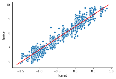
# let's plot our data with the OLS predicted fit
np.random.seed(40)
sns.scatterplot(x='lcarat',y='lprice',data=diamonds2.sample(1000)) # sampled just to avoid overplotting
sns.lineplot(x=diamonds2['lcarat'],y=y_predicted1,color='red')
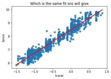
# compare this to the built-in sns produces
plt.show()
np.random.seed(40)
sns.regplot(x='lcarat',y='lprice',data=diamonds2.sample(1000),
line_kws={'color':'red'}).set_title("Which is the same fit sns will give")
Example: Including dummy variables
Suppose you started by estimating the price of diamonds as a function of carats
\begin{align} \log(\text{price})=a+\beta_0 \log(\text{carat}) +u \end{align}but you realize it will be different for ideal cut diamonds. That is, a 1 carat diamond might cost $1,000, but if it's ideal, it's an extra $500 dollars.
\begin{align} \log(\text{price})= \begin{cases} a+\beta_0 \log(\text{carat}) + \beta_1 +u, & \text{if ideal cut} \\ a+\beta_0 \log(\text{carat}) +u, & \text{otherwise} \end{cases} \end{align}Notice that $\beta_0$ in this model are the same. Here is how you run this test:
# ideal is a dummy variable = 1 if ideal and 0 if not ideal
model_ideal   = sm_ols('lprice ~ lcarat + ideal', data=diamonds2)
results_ideal = model_ideal.fit()               # estimate / fit
print(results_ideal.summary())             # view results
sm_ols('lprice ~ cut', data=diamonds2).fit().summary()
Example: Including interaction terms
Suppose that an ideal cut diamond doesn't just add a fixed dollar value to the diamond. Perhaps it also changes the value of having a larger diamond. You might say that
- A high quality cut is even more valuable for a larger diamond than it is for a small diamond. ("A great cut makes a diamond sparkle, but it's hard to see sparkle on a tiny diamond no matter what.")
- In other words, the effect of carats depends on the cut and visa versa
- In other words, "the cut variable interacts with the carat variable"
- So you might say that, "a better cut changes the slope/coefficient of carat"
- Or equivalently, "a better cut changes the return on a larger carat"
Graphically, it's easy to see, as sns.lmplot by default gives each cut a unique slope on carats:
# notice how these lines have different slopes?
np.random.seed(40)
subsample_of_equal_amounts = diamonds2.query('cut in ["Ideal","Fair"]').groupby('cut').apply(lambda x: x.sample(400))
sns.lmplot(data=subsample_of_equal_amounts,
           y='lprice',x='lcarat',hue='cut',ci=None)
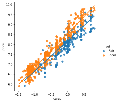
Those two different lines above are estimated by
\begin{align} \log(\text{price})= a+ \beta_0 \log(\text{carat}) + \beta_1 \text{Ideal} + \beta_2\log(\text{carat})\cdot \text{Ideal} \end{align}If you plug in 1 for $ideal$, you get the line for ideal diamonds as
\begin{align} \log(\text{price})= a+ \beta_1 +(\beta_0 + \beta_2) \log(\text{carat}) \end{align}If you plug in 0 for $ideal$, you get the line for fair diamonds as
\begin{align} \log(\text{price})= a+ \beta_0 \log(\text{carat}) \end{align}So, by including that interaction term, you get that the slope on carats is different for Ideal than Fair diamonds.
sm will estimate that nicely:
# you can include the interaction of x and z by adding "+x*z" in the spec, like:
sm_ols('lprice ~ lcarat + ideal + lcarat*ideal', data=subsample_of_equal_amounts).fit().summary()
This shows that a 1% increase in carats is associated with a 1.53% increase in price for fair diamonds, but a 1.72% increase for ideal diamonds (1.53+0.19).
Thus: The return on carats is different (and higher) for better cut diamonds!
Mechanical interpretation of regression coefficients
If X is a continuous variable
| If the model is.................. | then $\beta$ means (approx. in log cases) |
|---|---|
| $y=a+\beta X$ | If $X \uparrow $ 1 unit, then $y \uparrow$ by $\beta$ units |
| $\log y=a+\beta X$ | If $X \uparrow $ 1 unit, then $y \uparrow$ by about $100*\beta$%. (Exact: $100*(\exp(\beta)-1)$) |
| $y=a+\beta \log X$ | If $X \uparrow $ 1%, then $y \uparrow$ by about $\beta / 100$ units |
| $\log y=a+\beta \log X$ | If $X \uparrow $ 1%, then $y \uparrow$ by $\beta$% |
If X is a binary variable
This is a categorical or qualitative variable with two values (aka "dummy"). E.g. gender in Census data, and "ideal" above.
| If the model is.................. | then $\beta$ means |
|---|---|
| $y=a+\beta X$ | $y$ is $\beta$ units higher for cases when $X=1$ than when $X=0$. |
| $\log y=a+\beta X$ | $y$ is about $\beta$ % higher for cases when $X=1$ than when $X=0$. |
If X is a categorical variable
This is a categorical or qualitative variable with more than two values. E.g. "cut" in the diamonds dataset. In a regression, this ends up looking like
So you do is take the cut variable cut={Fair,Good,Very Good,Premium,Ideal} and turn it into a dummy variable for "Good", a dummy variable for "Very Good", and so on.
Warning: You don't create a dummy variable for all the categories! That's why I skipped "Fair" in the prior paragraph.
Then...
| $\beta$..... | means | or |
|---|---|---|
| $\beta_{Good}$ | The average log(price) for Good diamonds is $\beta_{Good}$ higher than Fair diamonds. | $avg_{Good}-avg_{Fair}$ |
| $\beta_{Very Good}$ | The average log(price) for Good diamonds is $\beta_{Very Good}$ higher than Fair diamonds. | $avg_{Very Good}-avg_{Fair}$ |
| $\beta_{Premium}$ | The average log(price) for Good diamonds is $\beta_{Premium}$ higher than Fair diamonds. | $avg_{Premium}-avg_{Fair}$ |
| $\beta_{Ideal}$ | The average log(price) for Good diamonds is $\beta_{Ideal}$ higher than Fair diamonds. | $avg_{Ideal}-avg_{Fair}$ |
THE MAIN THING TO REMEMBER IS THAT $\beta_{value}$ COMPARES THAT $value$ TO THE OMITTED CATEGORY!
So, compare the regression above which reports that $a$ (intercept) = 8.0688 and $\beta_{Good}$ equals -0.2328 to this:
diamonds2.groupby('cut')['lprice'].mean() # avg lprice by cut
8.0688 + (-0.2328) = 7.8360!!!
The nice part of sm is that it automatically "creates" the dummy variables and omits a value for you!
Interpreting with multiple variables (THE WOES THEREOF)
If you have multiple (up to N controls):
\begin{align} y = a +\beta_0 X_0 + \beta_1 X_1+ ...+\beta_N X_N+ u \end{align}- $\beta_1$ estimates the expected change in Y for a 1 unit increase in $X_1$ (as we covered above).
- But predictors usually change together!!!
If Y = number of tackles by a football player in a year, $W$ is weight, and $H$ is height, and we estimate that
\begin{align} y = a +\hat{0.5} W + \hat{-0.1} H \end{align}
How do you interpret $\hat{\beta_1} < 0 $ on H?
If categorical variables are included (e.g. year or industry), when thinking about the OTHER variables, you can think
- "comparing same firms within the same year..."
- "comparing firms in the same industry, controlling for industry factors..."
A useful trick: Comparing the size of two coefficients
Earlier, we estimated that $\log price = \hat{8.41} + \hat{1.69} \log carat + \hat{0.10} ideal$.
So... I have questions:
- Does that mean that $\log carat$ has a 17 times larger impact than $ideal$ in terms of price impact?
- How do we compare those magnitudes?
- More generally, how do we compare the magnitudes of any 2 control variables?
To which, I'd say that how "big" a coefficient is depends on the variable!
- For some variables, an increase of 1 unit is common (e.g. our $ideal$ dummy is one 40% of the time)
- For some variables, an increase of 1 unit is rare (e.g. leverage)
- $\rightarrow$ the meaning of the coefficient's magnitude depends on the corresponding variable's variation!
- $\rightarrow$ so change variables so that a 1 unit increase implies the same amount of movement
- $\rightarrow$ Solution: scale variables by their standard deviation!*
* (Only continuous variables! Don't do this for dummy variables or categorical variables)
Here is that solution in action:
standardize = lambda x:x/x.std() # normalize(df['x']) will divide all 'x' by the std deviation of 'x'

print("Divide lcarat by its std dev:\n")
print(sm_ols('lprice ~ lcarat + ideal',
       # for **just** this regression, divide
       data=diamonds2.assign(lcarat = standardize(diamonds2['lcarat']))
       # this doesn't change the diamonds2 data permanently, so the next time you call on
       # diamonds2, you can use lcarat as if nothing changed. if you want to repeat this
       # a bunch, you might instead create and save a permanent variable called "lcarat_std"
       # where "_std" indicates that you divided it by the std dev.
      ).fit().params)

print("\n\nThe original reg:\n")
print(sm_ols('lprice ~ lcarat + ideal',data=diamonds2 ).fit().params)
So a 1 standard deviation increase in $\log carat$ is associated with a 0.98% increase in price. Compared to $ideal$, we can say that a reasonable variation in carats is associated with a price increase about 10 times the size.
Notably, 0.98 is only 58% of the original coefficient (1.69).
Q: Why is it 58% of the previous coefficient?
A: Because the standard deviation of $\log carat$ is 0.58!
This works because, if "$std$" stands for the standard deviation of $\log carat$ each of these steps is valid and doesn't change the estimation:
\begin{align} \log price & = \hat{8.41} + \hat{1.69} \log carat + \hat{0.10} ideal \\ & = \hat{8.41} + \hat{1.69} \frac{std}{std} \log carat + \hat{0.10} ideal \\ & = \hat{8.41} + (\hat{1.69}*std) \frac{\log carat}{std} + \hat{0.10} ideal \end{align}So what that last line shows is that if we divide the variable by its standard deviation, the coefficient will change by an offsetting amount.
If a variable has a small standard deviation (e.g. 0.10), dividing the variable by 0.10 before running the regression will reduce the coefficient by 90%.
Here, $\log carat$ has a deviation of 0.58, so scaling the variable before regressing dropped the
Goodness of fit: R2 and Adjusted R2
The next graph shows two different y variables (shown in blue and orange). Each is "modelled" as a linear function of carats. After we run a regression, we get a prediction for each.
Which line/prediction do you think fits its corresponding data points better? Blue or orange?
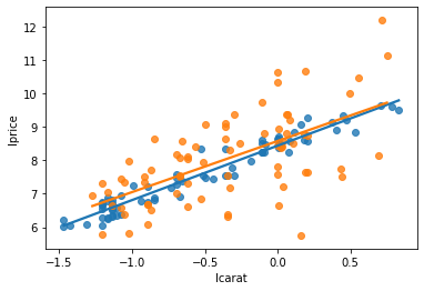
Intuitively, the line model "fits" the blue data much better! Your eyes can tell you that the blue data points are much more tightly bunched around the blue line than the orange dots and line are.
One way to summary that idea is via R2, aka "R-squared". R2 measures how much variation in the y variable is explained by the regression line, and ranges from 0 to 1. Every table above automatically reports R2.
But there are a two massive problems with R2:
- Including extra X variables can never decrease R2, and in fact, variables that are random noise can increase R2.
- Because of (1), optimizing on R2 will quickly lead to including X variables you probably shouldn't. In other words, it will lead to overfitting a model, which means designing a model so specifically to your existing data that it will apply poorly to new data.
This is why you should probably focus on looking at the Adjusted R2 in regressions, which is simply R2 with a penality for adding additional variables to the model.
Regression coefficients have "feelings"
OR: T-stats and P-Values
Well, not feelings, like bad or good but more like uncertainty.

The tables above report t-stats and p-values for statistics, which I'm only going to briefly review here. (I'm going to assume you are mostly familiar with these via your pre-reqs. Please let me know if I'm mistaken!)
A coefficient's t-stat and p-value can be used to assess the probability that the coefficient is different than zero by random chance.
- A t-stat of 1.645 corresponds to a p-value of 0.10; meaning only 10% of the time would you get that coefficient randomly
- A t-stat of 1.96 corresponds to a p-value of 0.05; this is a common "threshold" to say a "relationship is statistically significant" and that "the relationship between X and y is not zero"
- A t-stat of 2.58 corresponds to a p-value of 0.01
These thresholds are important and part of a sensible approach to learning from data, but...
When people say a "relationship is statistically significant", what they can mean is
CORRELATION THAT IS TRUE
(TRULY!) (VERILY!)
AND KNOWING IT WILL CHANGE THE WORLD!"
Which leads me to the next section.
Some significant warnings about "statistical significance"
The focus on p-values can be dangerous. As it turns out, "p-hacking" (finding a significant relationship) is easy for a number of reasons:
- If you look at enough Xs and enough ys, you, by chance alone, can find "significant" relationships where none exist
Your data can be biased. Maybe the most famous example:

The newspaper ran a telephone poll in 1948 and found a significant preference for Dewey. The problem? Phones were still expensive in 1948. Their polling method accounted for rural/urban and race, but not income.
Another bias that contributed? The paper had to publish earlier than others due to printing issues, so they used an expert who had been right in 4 of the last 5 elections.

Turns out a sample size of five wasn't enough to confirm the expert had a crystal ball.

The notion of turning to people on hot streaks has been pretty roundly debunked in finance (e.g. mutual funds, stock pickers, etc). But my favorite example is Paul the Octopus, who picked winners in all seven soccer matches Germany played during the 2010 World Cup.
Your sample restrictions can generate bias: If you evaluate the trading strategy "buy and hold current S&P companies" for the last 50 years, you'll discover that this trading strategy was unbelievable!
Reusing the data: If you torture the data, it will confess
There is a fun game in here. The point: The choices you make about what variables to include or focus on can change the statistical results. And if you play with a dataset long enough, you'll find "results"...
The focus on p-values can be dangerous because it distorts the incentives of researchers:
- Again: If you torture the data, it will confess (regardless of whether you or it wanted to)
- Motivated reasoning/cognitive dissonance/confirmation bias: Analysis like the game above is fraught with temptations for humans. That 538 article mentions that about 2/3 of retractions are due to misconduct.
- Focus on p-value shifts attention: Statistical signicance does not mean meaningful or economic significance

Reading / practice for this topic
- This page!
- Chapters 22-24 of R 4 Data Science are an excellent overview of the thought process of modeling
- Use
statsmodels.apito make nice regression tables by following this guide (you can use different data though) - Load the titanic dataset from
snsand try some regressions.