Intro to Pandas

Powerful Pandas

It's time to learn pandas.

I promise it will go better than this

... and when we're done,

I also promise: Only 3 more panda gifs this lecture.

Outline

Be patient and persistent: keep going when the scope of pandas and your first data analysis exercises stump you!
Essential functions for data wrangling, statistics, and exploration
Example: Data wrangling and exploration that is readable and powerful
Cookbook: Typical data analysis steps, table creation, and figures

Do not fret the size of Pandas

There are over 250 methods that work on DataFrames objects! This means two things:

(Unlimited) Power!
Oye, hard to remember!

On top of trying to memorize (well, sort of) the available methods, a tough part of data science is conceptualizing how to shape and format and construct datasets so that algos you want to run can run and so that plots can plot.

So I'm going to try to reduce it to the most common operations, and make you aware of things you can do. By the end of the semester, your Pandas proficiency will have you feeling like Sheev Palpy.

Until then, rely on this page, develop and save your "cookbooks" for common operations you run into.
Knowing about possible operations, and when and why to use them is more important than memorizing syntax! If you have a firm-year panel with sales, and you want to compute industry computation, knowing that you can run a groupby to reduce a firm-year panel to an industry-year panel is more important than knowing the groupby syntax. You can always look up syntax once you know a function is needed.
This chapter contains a lot of informational tables and code snippets; read it at least twice. Once to understand when and why to run a given function, and once to dig into the syntax.
I cover only the most essential functions. Make sure to bookmark pandas documentation (which is in Jupyter's "Help" menu too) and a favorite resource from the Resources tab.

Pandas is worth the overhead. This class as a whole is utterly unfeasible without pandas, as it makes cutting edge data science feasible (and easy, ultimately!). Additionally, it is the #1 way that professionals in industry and academia interact with tabular data in Python. (Read: Pandas get paid.)

Let me repeat: bookmark the pandas documentation, you'll be there a lot!

What is pandas / vocab

The fundamental principle of database design is that the physical structure of a database should communicate its logical structure

Pandas data are stored in two-dimensional tables that do this. A few vocabulary terms:

"Index" - The identifying information for a row. In our "Golden Rules" lecture we used the term "key" (which I prefer), but pandas uses Index.
"Series" - A database with a single column ("variable")
"DataFrame" - A database with as many columns/variables as you'd like (0, 1, ... 1 million). A DataFrame is, in essence, an Excel sheet.
"Wide data" vs. "Long data":

The notion of "wide" and "long" data still applies when more variables are added:

This is a long dataset:

Year	Firm	Sales	Profits
2000	Ford	10	1
2001	Ford	12	1
2002	Ford	14	1
2003	Ford	16	1
2000	GM	11	0
2001	GM	13	2
2002	GM	13	0
2003	GM	15	2

The exact same data, stored as a wide dataset:

Year	Sales GM	Ford	Profits GM	Ford
2000	11	10	0	1
2001	13	12	2	1
2002	13	14	0	1
2003	15	16	2	1

This is a long dataset, or a "tall" dataset:

Year	Firm	Sales
2000	Ford	10
2001	Ford	12
2002	Ford	14
2003	Ford	16
2000	GM	11
2001	GM	13
2002	GM	13
2003	GM	15

The exact same data, stored as a wide dataset:

Year	Sales GM	Ford
2000	11	10
2001	13	12
2002	13	14
2003	15	16

Notice here how the variables have multiple levels for the variable name: level 0 is "Sales" which applies to the level 1 "GM" and "Ford". Thus, column 2 is Sales of GM and column 3 is Sales of Ford.

You will need to get comfortable with "MultiIndex", as pandas calls these.

The essential data wrangling toolkit

I imagine you'll return to this page a lot. Today and tomorrow,

I'm going to make note of a few important tools we have available
I'll show you an example that illustrates how those tools can be applied
We'll practice together
You'll be in position to attack ASGN 02
Over time and with experience, pandas will become less overwhelming and more of a friend!

Note 1: "df" is often used as a name of a generic dataframe in examples. Generally, you should give your dataframes better names!

Note 2: There are other ways to do many of these operations. For example (the sidebar illustrates)

df['feet']=df['height']//12 will create a new column called feet
df[['gender','height']] will return just those two columns-
df.loc[df['feet']==5,'feet'] = np.nan will overwrite the feet variable only when feet equals 5
More on indexing and selection here---highly recommend! If that link is dead: https://jakevdp.github.io/PythonDataScienceHandbook/03.02-data-indexing-and-selection.html

import pandas as pd # everyone imports pandas as pd
import numpy as np
df = pd.DataFrame({'height':[72,60,68],'gender':['M','F','M'],'weight':[175,110,150]})

df['feet']=df['height']//12
print("\n\n Original df:\n",df) 
print("\n\n Subset of vars:\n",df[['gender','height']])
df.loc[df['feet']==5,'feet'] = np.nan
print("\n\n Replace given condition:\n",df)


 Original df:
    height gender  weight  feet
0      72      M     175     6
1      60      F     110     5
2      68      M     150     5


 Subset of vars:
   gender  height
0      M      72
1      F      60
2      M      68


 Replace given condition:
    height gender  weight  feet
0      72      M     175   6.0
1      60      F     110   NaN
2      68      M     150   NaN

Essential `pandas`: Manipulating data

Try to notice, throughout this lecture, when methods operate on specific DataFrames (e.g. assign) and when methods are a called on the pandas module itself (e.g. pd.merge). Generally, methods that work outside a single DataFrame (the load data or work on multiple datasets) are called via pd.<method> while methods that work on a single DataFrame are called via <dfname>.<method>.

Function	Pandas method	Example
new variables or replace existing	assign	`df.assign(feet=df['height']//12)`
get subset of columns	filter	`df.filter(['height','weight'])`
rename columns	rename	`df.rename(columns={"height": "how tall"})`
get subset of observations or, "drop rows"	query / loc / iloc	`df.query('height > 68')` `df.loc[df['gender']=='F']` `df.iloc[1:]`
sort	sort_values	`df.sort_values(['gender','weight'])`
create groups	groupby	`df.groupby(['gender'])`
summary stats on groups	agg / pivot_table	`df.groupby(['gender'])` `.agg({'height':[max,min,np.mean]})` `df.pivot_table(index='age', columns='age', values='weight'`
create a variable based on its group	agg+transform	`df.groupby(['industry','year'])['leverage'].mean().transform()` will add industry average leverage to your dataset for each firm
delete column	drop	`df.drop(columns=['gender'])`
use non-pd function on df	pipe	`df.pipe((sns.lineplot,data),x=x,y=y)`
combine dataframes	merge	`pd.merge(df1,df2)`
RESHAPE: convert wide to long/tall ("stack!")	stack	`df.stack()`, see popout
... another option to reshape tall:	melt
RESHAPE: convert long/tall to wide ("unstack!")	unstack	`df.unstack()`, see popout
... another option to reshape wide:	pivot / pivot_table
change time frequency of data	resample	`df.resample('Y').mean()`
loading data	read_csv, read_dta, etc	`pd.read_csv('wine.csv')`
window/rolling calculations	window	`df['vol_5yr']= df.groupby('firm').rolling(36).var('ret').transform()` will add 36 period volatility for each firm

When you wonder about syntax, and arguments, you can either go to the official documentation on the web, or rely on Jupyter's tab auto completion.

Here is a fun trick: SHIFT+TAB! Try it! Type import pandas as pd then run that to load pandas. Then type pd.merge( like you want to merge to dataframes, except you don't remember the arguments to use. So type SHIFT+TAB+TAB. 1 TAB opens a little syntax screen, 2 opens a larger amount of syntax info, and 3 opens the whole help file at the bottom of the screen. I've personally moved to SHIFT+TAB for help most of the time (instead of help() or ?).

# AN ASIDE ON RESHAPING

df = pd.Series({   ('Ford',2000):10,
                   ('Ford',2001):12,
                   ('Ford',2002):14,
                   ('Ford',2003):16,
                   ('GM',2000):11,
                   ('GM',2001):13,
                   ('GM',2002):13,
                   ('GM',2003):15}).to_frame().rename(columns={0:'Sales'}).rename_axis(['Firm','Year'])
print("Original:\n",df)
wide = df.unstack(level=0)
print("\n\nUnstack (make it shorter+wider)\non level 0/Firm:\n",wide) # move index level 0 (firm name) to column
tall = wide.stack()
print("\n\nStack it back (make it tall):\n",tall) # move index level 0 (firm name) to column
print("\n\nStack it back and reorder \nindex as before (firm-year):\n",tall.swaplevel().sort_index())

print("\n\nUnstack level 1/Year:\n",df.unstack(level=1)) # move index level 0 (firm name) to column

Original:
            Sales
Firm Year       
Ford 2000     10
     2001     12
     2002     14
     2003     16
GM   2000     11
     2001     13
     2002     13
     2003     15


Unstack (make it shorter+wider)
on level 0/Firm:
      Sales    
Firm  Ford  GM
Year          
2000    10  11
2001    12  13
2002    14  13
2003    16  15


Stack it back (make it tall):
            Sales
Year Firm       
2000 Ford     10
     GM       11
2001 Ford     12
     GM       13
2002 Ford     14
     GM       13
2003 Ford     16
     GM       15


Stack it back and reorder 
index as before (firm-year):
            Sales
Firm Year       
Ford 2000     10
     2001     12
     2002     14
     2003     16
GM   2000     11
     2001     13
     2002     13
     2003     15


Unstack level 1/Year:
      Sales               
Year  2000 2001 2002 2003
Firm                     
Ford    10   12   14   16
GM      11   13   13   15

Temp vs. Permanent Methods

This is generally true with python but I'll reiterate here: Using methods on an object (e.g. a DataFrame) will give you an object with the method applied, as you can see here:

# define a df
df = pd.DataFrame({'height':[72,60,68],'gender':['M','F','M'],'weight':[175,110,150]})
# call method on df and print
print( df.assign(feet=df['height']//12))

   height gender  weight  feet
0      72      M     175     6
1      60      F     110     5
2      68      M     150     5

Which is useful if you want to alter the variable temporarily (e.g. for a graph, or to just print it out, like I literally just did!).

But the object in memory wasn't changed when I used df.<method>. See, here is the df in memory:

print(df)  # see, no feet!

   height gender  weight
0      72      M     175
1      60      F     110
2      68      M     150

If you want to change the object permanently, you have three options:

# option 1: explicitly define the df as the prior df after the method was called
df = df.assign(feet1=df['height']//12) 

# option 2: define a new feature of the df
df['feet2']=df['height']//12

# option 3: some methods have an "inplace" option so you don't need to write "df = ..."
df.drop(columns='gender',inplace=True)

print(df) # feet1 and feet 2 added to obj in memory, gender dropped

   height  weight  feet1  feet2
0      72     175      6      6
1      60     110      5      5
2      68     150      5      5

Generally, option 2 > 1 (it is easier to read), but you'll need to use option 1 when you're method chaining.

Essential `pandas`: Statistical operations

These functions can be called for a variable "col1" in this form: df['col1'].<function>() or for all numerical columns at once using df.<function>().

ALSO: These functions work within groups.

Function	Description
count	Number of non-null observations
sum	Sum of values
mean	Mean of values
mad	Mean absolute deviation
median	Arithmetic median of values
min	Minimum
max	Maximum
mode	Mode
abs	Absolute Value
prod	Product of values
std	Unbiased standard deviation
var	Unbiased variance
sem	Unbiased standard error of the mean
skew	Unbiased skewness (3rd moment)
kurt	Unbiased kurtosis (4th moment)
quantile	Sample quantile (value at %)
cumsum	Cumulative sum
cumprod	Cumulative product
cummax	Cumulative maximum
cummin	Cumulative minimum
nunique	How many unique values?
value_counts	How many of each unique value are there?

Essential `pandas`: Exploring the dataset

You should always, always, always open your datasets up to physically (digitally?) look at them and then also generate summary statistics:

Print the first and last five rows: df.head() and df.tail()
What is the shape of the data? df.shape
How much memory does it take, and what are the variable names/types? df.info()
Summary stats on variables: df.describe(), df.value_counts[:10], and df['var'].nunique()

Consider these Golden Rules.

# import a famous dataset, seaborn nicely contains it out of the box!
import seaborn as sns 
iris = sns.load_dataset('iris') 

print(iris.head())
print(iris.tail())
print("\n\nThe shape is: ",iris.shape)
print("\n\nInfo:",iris.info()) # memory usage, name, dtype, and # of non-null obs (--> # of missing obs) per variable
print(iris.describe()) # summary stats, and you can customize the list!

   sepal_length  sepal_width  petal_length  petal_width species
0           5.1          3.5           1.4          0.2  setosa
1           4.9          3.0           1.4          0.2  setosa
2           4.7          3.2           1.3          0.2  setosa
3           4.6          3.1           1.5          0.2  setosa
4           5.0          3.6           1.4          0.2  setosa
     sepal_length  sepal_width  petal_length  petal_width    species
145           6.7          3.0           5.2          2.3  virginica
146           6.3          2.5           5.0          1.9  virginica
147           6.5          3.0           5.2          2.0  virginica
148           6.2          3.4           5.4          2.3  virginica
149           5.9          3.0           5.1          1.8  virginica


The shape is:  (150, 5)
<class 'pandas.core.frame.DataFrame'>
RangeIndex: 150 entries, 0 to 149
Data columns (total 5 columns):
sepal_length    150 non-null float64
sepal_width     150 non-null float64
petal_length    150 non-null float64
petal_width     150 non-null float64
species         150 non-null object
dtypes: float64(4), object(1)
memory usage: 6.0+ KB


Info: None
       sepal_length  sepal_width  petal_length  petal_width
count    150.000000   150.000000    150.000000   150.000000
mean       5.843333     3.057333      3.758000     1.199333
std        0.828066     0.435866      1.765298     0.762238
min        4.300000     2.000000      1.000000     0.100000
25%        5.100000     2.800000      1.600000     0.300000
50%        5.800000     3.000000      4.350000     1.300000
75%        6.400000     3.300000      5.100000     1.800000
max        7.900000     4.400000      6.900000     2.500000

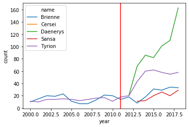
Game of Thrones example - slicing, group stats, and plotting

I didn't find an off the shelf dataset to run our seminal analysis from last week, but I found an analysis that explored if Game of Thrones prompted parents to start naming their children differently. The following is inspired by that, but uses pandas to acquire and wrangle our data in a "Tidyverse"-style (how R would do it) flow.

#TO USE datadotworld PACKAGE:
#1. create account at data.world, then run the next two lines:
#2. in terminal/powershell: pip install datadotworld[pandas]
#
#   IF THIS DOESN'T WORK BC YOU GET AN ERROR ABOUT "CCHARDET", RUN:
#    conda install -c conda-forge cchardet
#   THEN RERUN: pip install datadotworld[pandas] 
#
#3. in terminal/powershell: dw configure          
#3a. copy in API token from data.world (get from settings > advanced)

import datadotworld as dw
import numpy as np
import pandas as pd
import seaborn as sns
import matplotlib.pyplot as plt

baby_names = dw.load_dataset('nkrishnaswami/us-ssa-baby-names-national')
baby_names = baby_names.dataframes['names_ranks_counts']

Version 1

save a slice of the dataset with the names we want (using .loc)
sometimes a name is used by boys and girls in the same year, so combine the counts so that we have one observation per name per year
save the dataset and then call a plot function

# restrict by name and only keep years after 2000
somenames = baby_names.loc[( # formating inside this () is just to make it clearer to a reader
    ( # condition 1: one of these names, | means "or"
        (baby_names['name'] == "Sansa") | (baby_names['name'] == "Daenerys") | 
        (baby_names['name'] == "Brienne") | (baby_names['name'] == "Cersei") | (baby_names['name'] == "Tyrion") 
    ) # end condition 1
    & # & means "and"
    ( # condition 2: these years
        baby_names['year'] >= 2000) # end condition 2
    )]

# if a name is used by F and M in a given year, combine the count variable
# Q: why is there a "reset_index"? 
# A: groupby automatically turns the groups (here name and year) into the index
#    reset_index makes the index simple integers 0, 1, 2 and also
#    turns the the grouping variables back into normal columns
# A2: instead of reset_index, you can include `as_index=False` inside groupby!
#     (I just learned that myself!)
somenames_agg = somenames.groupby(['name','year'])['count'].sum().reset_index().sort_values(['name','year'])

# plot
sns.lineplot(data=somenames_agg, hue='name',x='year',y='count')
plt.axvline(2011, 0,160,color='red') # add a line for when the show debuted

<matplotlib.lines.Line2D at 0x2dd2103ad48>

Version 2 - `query` > `loc`, for readability

Same as V1, but step 1 uses .query to slice inside of .loc

save a slice of the dataset with the names we want (using .query)
sometimes a name is used by boys and girls in the same year, so combine the counts so that we have one observation per name per year
save the dataset and then call a plot function

# use query instead to slice, and the rest is the same
somenames = baby_names.query('name in ["Sansa","Daenerys","Brienne","Cersei","Tyrion"] & \
         year >= 2000') # this is one string with ' as the string start/end symbol. Inside, I can use 
                        # normal quote marks for strings. Also, I can break it into multiple lines with \
somenames_agg = somenames.groupby(['name','year'])['count'].sum().reset_index().sort_values(['name','year'])
sns.lineplot(data=somenames_agg, hue='name',x='year',y='count')
plt.axvline(2011, 0,160,color='red') # add a line for when the show debuted

<matplotlib.lines.Line2D at 0x2dd1e387bc8>

Version 3 - Method chaining!

Method chaining: Call the object (baby_names) and then keep calling one method on it after another.

Python will call the methods from left to right.
There is no need to store the intermediate dataset (like somenames and somenames_agg above!)
- --> Easier to read and write without "temp" objects all over the place
- You can always save the dataset at an intermediate step if you need to

So, the first two steps are the same, just the methods will be chained. And then, a bonus trick to plot without saving.

Slice with .query to GoT-related names
Combine M and F gender counts if a name is used by both in the same year
Plot without saving: "Pipe" in the plotting function

The code below produces a plot identical to V1 and V2, but it is unreadable. Don't try - I'm about to make this readable! Just one more iteration...

baby_names.query('name in ["Sansa","Daenerys","Brienne","Cersei","Tyrion"] & year >= 2000').groupby(['name','year'])['count'].sum().reset_index().pipe((sns.lineplot, 'data'),hue='name',x='year',y='count')
plt.axvline(2011, 0,160,color='red') # add a line for when the show debuted

<matplotlib.lines.Line2D at 0x2dd1f726308>

To make this readable, we write a parentheses over multiple lines

(
    and python knows to execute the code inside as one line
)

And as a result, we can write a long series of methods that is comprehensible, and if we want we can even comment on each line:

(baby_names
      .query('name in ["Sansa","Daenerys","Brienne","Cersei","Tyrion"] & \
         year >= 2000')
      .groupby(['name','year'])['count'].sum() # for each name-year, combine M and F counts
      .reset_index() # give us the column names back as they were (makes the plot call easy)
      .pipe((sns.lineplot, 'data'),hue='name',x='year',y='count')
)    
plt.axvline(2011, 0,160,color='red') # add a line for when the show debuted
plt.title("WOW THAT WAS EASY TO WRITE AND SHARE")

Text(0.5, 1.0, 'WOW THAT WAS EASY TO WRITE AND SHARE')

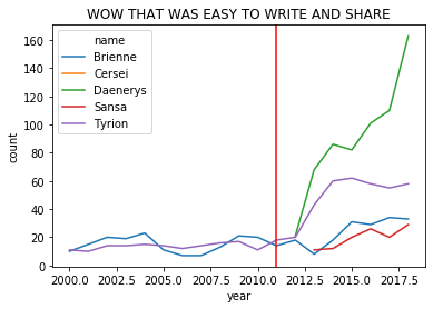
WOW. That's nice code!

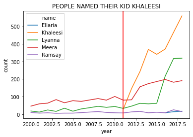
Also: Naming your baby Daenerys after the hero...

...is a bad break.

(baby_names
      .query('name in ["Khaleesi","Ramsay","Lyanna","Ellaria","Meera"] & \
         year >= 2000')
      .groupby(['name','year'])['count'].sum() # for each name-year, combine M and F counts
      .reset_index() # give use the column names back as they were (makes the plot call easy)
      .pipe((sns.lineplot, 'data'),hue='name',x='year',y='count')
)    
plt.axvline(2011, 0,160,color='red') # add a line for when the show debuted
plt.title("PEOPLE NAMED THEIR KID KHALEESI")

Text(0.5, 1.0, 'PEOPLE NAMED THEIR KID KHALEESI')

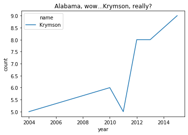
BUT IT COULD BE WORSE

(baby_names
      .query('name in ["Krymson"] & year >= 1950')
      .groupby(['name','year'])['count'].sum() # for each name-year, combine M and F counts
      .reset_index() # give use the column names back as they were (makes the plot call easy)
      .pipe((sns.lineplot, 'data'),hue='name',x='year',y='count')
)    
plt.title("Alabama, wow...Krymson, really?")

Text(0.5, 1.0, 'Alabama, wow...Krymson, really?')

Cookbook and best practices (a starter kit)

General analysis steps and comments

Start with the basic data exploration steps above
- variable names, types, count/missing, distributions
Data cleaning:
- Do some variables have large outliers? You might need to winsorize or drop those observations.
- Do some variables have many missing variables? Maybe there was a problem with the source or how you loaded it.
- Do some variables have impossible values? For example, sales can't be negative! Yet, some datasets use "-99" to indicate missing data. Or are there bad dates (June 31st)?
- Are there duplicate observations (e.g. two 2001-GM observations because they changed their fiscal year in the middle of calendar year 2001?)
- Are there missing observations or a gap in the time series (e.g. no observation in 2005 for Enron because the executive team was too "distracted to file its 10-K)
- Do variables contradict each other? (E.g. If my birthday is 1/5/1999, then I must be 21 as of this writing.)
Institutional knowledge is crucial.
- For example, in my research on firm investment policies and financing decisions (e.g. leverage), I drop any firms from the finance or utility industries. I know to do this because those industries are subject to several factors that fundamentally change their leverage in ways unrelated to their investment policies. Thus, including them would contaminate any relationships I find.
- When we work with 10-K text data, we need to know what data tables are available and how to remove boilerplate.
- You only get institutional through reading supporting materials, documentation, related info (research papers and WSJ, etc), and... the documents themselves. For example, I've read in excess of 6,000 proxy statements for a single research project. (If that sounds exciting: Go to grad school and become a prof!)
Explore the data with your question in mind
- Compute statistics by subgroups (by age, or industry), or two-way (by gender and age)
- This step reinforces institutional knowledge and understanding of the data
- Data exploration and data cleaning are interrelated and you'll go back and forth from one to the other.

Creating summary tables

A big part of the challenge is knowing what "cuts" of the data are interesting. You'll figure this out as you get more knowledge in a specific area.
In tables that cut data based on two variables, how do you decide on the "second variable" to slice?
1. Secondary slices might be on a priori (known in advance) interesting variables ("everyone talks about growth potential so I'll also cut by that too because they will wonder about it if I don't")
2. Or, choose second variables because you think that the impact of the first variable will depend on the second variable. Suppose you divide firms into "young and old" as a first slice. Your second slice might be industries: perhaps leverage is only a little lower for older railroad firms but leverage is much higher for large firms in tech industries.
3. Another example: A common data science training dataset is about surviving the Titanic. Women survived at higher rates, but this is especially true in first class, where very few women died. The gender disparity was less severe in third class; while third class men were more likely to perish than first class men, 45% of women in third class died, compared to ~0 in first class.

Essential reading. Rather than me replicating these pages, read these after class, follow them, and save snippets of code you find useful to your growing cheat sheet.

Creating summary plots

Next week! But you'll see a little plotting in the practice session. Speaking of which...

Time to practice

Inside the Lecture repo, go into the 02 subfolder and find the 02a-pandas-practice.ipynb file and download it to your participation repo.

HINTS and supporting examples: See the links a few lines above this!

Before next class

Finish and upload the numpy and pandas practice files to your participation repo.
Read the Aggregation and grouping and Pivot tables links
Peer reviews are due tomorrow and an assignment on Monday!

Credits

Here are some links I found that I liked. They cover many aspects of pandaing:

This covers indexing and slicing issues nicely
This covers method chaining so that Python can approximate R's elegance at data wrangling and plotting
This also has nice and quick examples showing Python matching R functions
The most popular questions about pandas on Stackoverflow. This will give you an idea of common places others get stuck, and slicing and indexing issues are high on the list.
https://www.textbook.ds100.org