Search
A Simple Program

A simple program (Yes, this webpage is a .ipynb file!)

The goal of this notebook is to illustrate basic finance computations within a markdown document. There is an analogous .py file, whose results have to be logged. Then, to produce output, you'd have to copy and paste key output into a Word document. This notebook does both at once!

The point of this notebook is ONLY illustration! Pay attention to its structure and flow, and get an early glimpse of just a little bit that we can do with pandas, seaborn, and a few other packages.

First, we start by importing key packages...

The core Python language is quite small (nimble and easy to maintain), so we add functionality by using external packages. The import calls should always be at the top of your code!

If you want to run this code (and you should try!)

  1. Download the raw raw unrendered ipynb file here called "02a-a-simple-program.ipynb". On Chrome and Firefox, you simply right click the file name and select "Save Link As". Put the file in the same folder with the file you're working on already and then open it in Jupyter.
  2. Open a new/second terminal/powershell and type pip install pandas_datareader
  3. Click the "Kernel" menu above, then "Restart & Clear Output". Now all the results below will disappear.
  4. Click the "Cell" menu above, then "Run All"
import pandas as pd
import numpy as np
import pandas_datareader as pdr # you might need to install this (see above)
import matplotlib.pyplot as plt
import seaborn as sns
import statsmodels.api as sm

Data

Pandas can acquire a lot of economic data itself, by downloading data from websites through built-in APIs. You'll learn what this means soon!

First, we grab stock prices for three fims. Then we compute daily returns and output some basic statistics.

stock_prices = pdr.get_data_yahoo(['AAPL','MSFT','VZ'], start=2006)
stock_prices = stock_prices.filter(like='Adj Close') # reduce to just columns with this in the name
stock_prices.columns = ['AAPL','MSFT','VZ']

daily_pct_change = pd.DataFrame()
for stock in ['AAPL','MSFT','VZ']:
    daily_pct_change[stock] = stock_prices[stock].pct_change() 

print(daily_pct_change.describe())
              AAPL         MSFT           VZ
count  3529.000000  3529.000000  3529.000000
mean      0.001195     0.000736     0.000503
std       0.019993     0.016712     0.013019
min      -0.179195    -0.117131    -0.080686
25%      -0.008105    -0.007089    -0.006257
50%       0.000952     0.000459     0.000701
75%       0.011256     0.008471     0.007201
max       0.139049     0.186047     0.146324

Data visualization - Compare the returns of sample firms

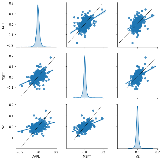
The following figure reports all of the pairwise correlations between the sample firms, along with the distribution of each.

We know from the above table that Apple has the largest mean and standard deviation of the three. The plot type below is useful for seeing if the variables have non-linear relationships, strange outliers, fat tails, or other issues.

# we need this helper function for a plot

def plot_unity(xdata, ydata, **kwargs):
    '''
    Adds a 45 degree line to the pairplot for plots off the diagonal
    
    Usage: 
    grid=sns.pairplot( <call pairplot as you want >  )
    grid.map_offdiag(plot_unity)
    '''
    mn = min(xdata.min(), ydata.min())
    mx = max(xdata.max(), ydata.max())
    points = np.linspace(mn, mx, 100)
    plt.gca().plot(points, points, color='k', marker=None,
            linestyle='--', linewidth=1.0)
     
# compare the return distribution of 3 firms visually...
    
grid = sns.pairplot(daily_pct_change,diag_kind='kde',kind="reg")
grid.map_offdiag(plot_unity) # how cool is that!
C:\Users\DoLe\Anaconda3\lib\site-packages\statsmodels\nonparametric\kde.py:447: RuntimeWarning: invalid value encountered in greater
  X = X[np.logical_and(X > clip[0], X < clip[1])] # won't work for two columns.
C:\Users\DoLe\Anaconda3\lib\site-packages\statsmodels\nonparametric\kde.py:447: RuntimeWarning: invalid value encountered in less
  X = X[np.logical_and(X > clip[0], X < clip[1])] # won't work for two columns.
<seaborn.axisgrid.PairGrid at 0xc950048>

Factor loadings

A core task in asset pricing is calculating the beta of a stock, along with loadings on other factors. The canonical model is the Fama-French 3 factor model, though 4 and 5 factor models are more popular nowadays.

Merge data on factor loadings with stock return data

We start by grabbing factor returns from Ken French's website, again via pandas API.

ff = pdr.get_data_famafrench('F-F_Research_Data_5_Factors_2x3_daily',start=2006)[0] # the [0] is because the imported obect is a dictionary, and key=0 is the dataframe
ff.rename(columns={"Mkt-RF":"mkt_excess"}, inplace=True) # cleaner name
ff = ff.join(daily_pct_change,how='inner') # merge with stock returns
for stock in ['MSFT','AAPL','VZ']:    
    ff[stock] = ff[stock] * 100 # FF store variables as percents, so convert to that
    ff[stock+'_excess'] = ff[stock] - ff['RF'] # convert to excess returns in prep for regressions
#print(ff.describe()) # ugly...
pd.set_option('display.float_format', lambda x: '%.2f' % x) # show fewer digits
pd.options.display.max_columns = ff.shape[1] # show more columns
print(ff.describe(include = 'all')) # better!
       mkt_excess     SMB     HML     RMW     CMA      RF    AAPL    MSFT  \
count     3502.00 3502.00 3502.00 3502.00 3502.00 3502.00 3501.00 3501.00   
mean         0.04    0.00   -0.01    0.01    0.00    0.00    0.12    0.07   
std          1.20    0.57    0.66    0.36    0.31    0.01    2.00    1.68   
min         -8.95   -3.40   -4.24   -2.62   -1.74    0.00  -17.92  -11.71   
25%         -0.40   -0.33   -0.31   -0.19   -0.18    0.00   -0.82   -0.71   
50%          0.08    0.00   -0.03    0.01   -0.01    0.00    0.09    0.04   
75%          0.56    0.33    0.26    0.21    0.17    0.01    1.12    0.85   
max         11.35    4.49    4.83    1.95    1.96    0.02   13.90   18.60   

           VZ  MSFT_excess  AAPL_excess  VZ_excess  
count 3501.00      3501.00      3501.00    3501.00  
mean     0.05         0.07         0.11       0.05  
std      1.31         1.68         2.00       1.31  
min     -8.07       -11.71       -17.93      -8.07  
25%     -0.63        -0.72        -0.82      -0.63  
50%      0.07         0.04         0.09       0.07  
75%      0.72         0.85         1.12       0.72  
max     14.63        18.60        13.90      14.63  

Now we run the models.

We loop over the stocks, and for each stock, we regress the stock's excess returns on a market (excess) return factor, the size factor "SMB" and the value factor "HML" (see Fama and French (1993)).

# run the models- 
params=pd.DataFrame()
for stock in ['MSFT','AAPL','VZ']:        
    print('\n\n\n','='*40,'\n',stock,'\n','='*40,'\n')
    model = sm.formula.ols(formula = stock+"_excess ~ mkt_excess + SMB + HML", data = ff).fit()
    print(model.summary())
    params[stock] = model.params.tolist()
params.set_index(model.params.index,inplace=True)   


 ======================================== 
 MSFT 
 ======================================== 

                            OLS Regression Results                            
==============================================================================
Dep. Variable:            MSFT_excess   R-squared:                       0.533
Model:                            OLS   Adj. R-squared:                  0.533
Method:                 Least Squares   F-statistic:                     1331.
Date:                Fri, 10 Jan 2020   Prob (F-statistic):               0.00
Time:                        14:21:56   Log-Likelihood:                -5442.2
No. Observations:                3501   AIC:                         1.089e+04
Df Residuals:                    3497   BIC:                         1.092e+04
Df Model:                           3                                         
Covariance Type:            nonrobust                                         
==============================================================================
                 coef    std err          t      P>|t|      [0.025      0.975]
------------------------------------------------------------------------------
Intercept      0.0236      0.019      1.217      0.224      -0.014       0.062
mkt_excess     1.1043      0.018     62.865      0.000       1.070       1.139
SMB           -0.3962      0.035    -11.221      0.000      -0.465      -0.327
HML           -0.4470      0.031    -14.398      0.000      -0.508      -0.386
==============================================================================
Omnibus:                      836.860   Durbin-Watson:                   2.005
Prob(Omnibus):                  0.000   Jarque-Bera (JB):            40286.368
Skew:                          -0.251   Prob(JB):                         0.00
Kurtosis:                      19.611   Cond. No.                         2.27
==============================================================================

Warnings:
[1] Standard Errors assume that the covariance matrix of the errors is correctly specified.


 ======================================== 
 AAPL 
 ======================================== 

                            OLS Regression Results                            
==============================================================================
Dep. Variable:            AAPL_excess   R-squared:                       0.380
Model:                            OLS   Adj. R-squared:                  0.379
Method:                 Least Squares   F-statistic:                     714.0
Date:                Fri, 10 Jan 2020   Prob (F-statistic):               0.00
Time:                        14:21:56   Log-Likelihood:                -6565.4
No. Observations:                3501   AIC:                         1.314e+04
Df Residuals:                    3497   BIC:                         1.316e+04
Df Model:                           3                                         
Covariance Type:            nonrobust                                         
==============================================================================
                 coef    std err          t      P>|t|      [0.025      0.975]
------------------------------------------------------------------------------
Intercept      0.0676      0.027      2.532      0.011       0.015       0.120
mkt_excess     1.0965      0.024     45.289      0.000       1.049       1.144
SMB           -0.1288      0.049     -2.647      0.008      -0.224      -0.033
HML           -0.4265      0.043     -9.969      0.000      -0.510      -0.343
==============================================================================
Omnibus:                      651.193   Durbin-Watson:                   1.940
Prob(Omnibus):                  0.000   Jarque-Bera (JB):            10938.202
Skew:                           0.389   Prob(JB):                         0.00
Kurtosis:                      11.624   Cond. No.                         2.27
==============================================================================

Warnings:
[1] Standard Errors assume that the covariance matrix of the errors is correctly specified.


 ======================================== 
 VZ 
 ======================================== 

                            OLS Regression Results                            
==============================================================================
Dep. Variable:              VZ_excess   R-squared:                       0.394
Model:                            OLS   Adj. R-squared:                  0.393
Method:                 Least Squares   F-statistic:                     757.6
Date:                Fri, 10 Jan 2020   Prob (F-statistic):               0.00
Time:                        14:21:56   Log-Likelihood:                -5024.3
No. Observations:                3501   AIC:                         1.006e+04
Df Residuals:                    3497   BIC:                         1.008e+04
Df Model:                           3                                         
Covariance Type:            nonrobust                                         
==============================================================================
                 coef    std err          t      P>|t|      [0.025      0.975]
------------------------------------------------------------------------------
Intercept      0.0213      0.017      1.236      0.217      -0.012       0.055
mkt_excess     0.6924      0.016     44.411      0.000       0.662       0.723
SMB           -0.3494      0.031    -11.150      0.000      -0.411      -0.288
HML            0.0805      0.028      2.923      0.003       0.027       0.135
==============================================================================
Omnibus:                      770.293   Durbin-Watson:                   1.910
Prob(Omnibus):                  0.000   Jarque-Bera (JB):            12316.887
Skew:                           0.603   Prob(JB):                         0.00
Kurtosis:                      12.109   Cond. No.                         2.27
==============================================================================

Warnings:
[1] Standard Errors assume that the covariance matrix of the errors is correctly specified.

Estimated factor loadings

pd.set_option('display.float_format', lambda x: '%.4f' % x) # show fewer digits
print(params)
              MSFT    AAPL      VZ
Intercept   0.0236  0.0676  0.0213
mkt_excess  1.1043  1.0965  0.6924
SMB        -0.3962 -0.1288 -0.3494
HML        -0.4470 -0.4265  0.0805

Plot the cumulative returns of the three stocks

Finally, I plot the cumulative return from January 1, 2006 until January 2020 by computing for each stock $i$

$cumret(i,T)=\prod^T_{t=0} (1+r_{i,t})$

where $T$ is a date and $t=0$ corresponds to the beginning of the sample.

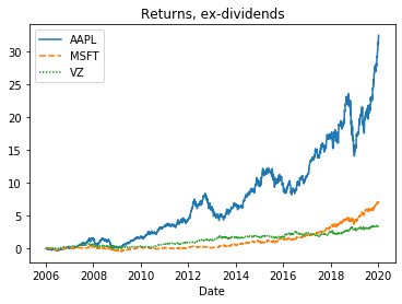
cumrets=(daily_pct_change+1).cumprod()-1
plt.clf() # clear the prior plot before starting a new one
sns.lineplot(data=cumrets).set_title("Returns, ex-dividends")
plt.show(grid)
C:\Users\DoLe\Anaconda3\lib\site-packages\pandas\plotting\_matplotlib\converter.py:103: FutureWarning: Using an implicitly registered datetime converter for a matplotlib plotting method. The converter was registered by pandas on import. Future versions of pandas will require you to explicitly register matplotlib converters.

To register the converters:
	>>> from pandas.plotting import register_matplotlib_converters
	>>> register_matplotlib_converters()
  warnings.warn(msg, FutureWarning)

Lecture flow

Now please go back and finish the lecture.