3.3.4. Visual EDA¶

The first page of this chapter discussed the reasons we plot our data.

Data cleaning: To find issues in the data that need to get fixed before we can do larger analysis
Data exploration: Learning about each of the variables, how they covary, and what further questions you can ask of the data
Analysis and presentation

3.3.4.1. EDA on a classic firm financial dataset¶

In the Pandas EDA page, I explored Compustat by producing summary stats to get a sense of the variables involved, look for missing values, and look for problematic outliers. We noted that some variables, like \(delaycon\), had a lot of missing values and decided we’d look into it.

Let’s continue exploring that dataset. First, let’s download our slice of it. The variables are listed and described in a csv file in the repo’s data folder.

import pandas as pd
import numpy as np
import matplotlib.pyplot as plt
import seaborn as sns
# these three are used to download the file
from io import BytesIO
from zipfile import ZipFile
from urllib.request import urlopen

url = 'https://github.com/LeDataSciFi/ledatascifi-2021/blob/main/data/CCM_cleaned_for_class.zip?raw=true'

#firms = pd.read_stata(url)   
# <-- that code would work, but GH said it was too big and
# forced me to zip it, so here is the work around to download it:

with urlopen(url) as request:
    data = BytesIO(request.read())

with ZipFile(data) as archive:
    with archive.open(archive.namelist()[0]) as stata:
        ccm = pd.read_stata(stata)

3.3.4.2. The mystery of the poorly populated variables¶

Again, there are some variables with lots of missing values.

(
    ( # these lines do the calculation - what % of missing values are there for each var
        ccm.isna()      # ccm.isna() TURNS every obs/variable = 1 when its missing and 0 else
       .sum(axis=0)     # count the number of na for each variable (now data is 1 obs per column = # missing)
        /len(ccm)       # convert # missing to % missing 
        *100            # report as percentage
    ) 
    # you can stop here and report this...
    # but I wanted to format it a bit...
    .sort_values(ascending=False)[:13]
    .to_frame(name='% missing') # the next line only works on a frame, and because pandas sees only 1 variable at this pt
    .style.format("{:.1f}")     # in the code, it calls this a "series" type object, so convert it to dataframe type object
)
#

	% missing
privdelaycon	74.4
debtdelaycon	74.4
equitydelaycon	74.4
delaycon	74.4
prodmktfluid	60.4
tnic3tsimm	56.5
tnic3hhi	56.5
largetaxlosscarry	33.5
smalltaxlosscarry	33.5
invopps_FG09	13.0
short_debt	12.8
sales_g	11.8
l_laborratio	10.4

When variables missing that much in a dataset, something systematic is going on and you need to figure it out.

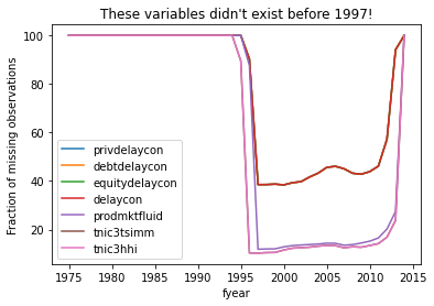
One way you could investigate why those variables are missing. Maybe it’s a data issue, as if some data for variable \(x\) isn’t available in all years. E.g. perhaps a variable isn’t available before 1995 for some reason.

A way you could get a start on that is to plot the % missing by year for each variable. This legend is UGGGGLY, because the plot has 40+ series, which is why it’s a spaghetti chart. It would take extra work to unravel the spaghetti and figure out what variables are what. But CLEARLY some variables only become available in 1995 so they can be used after that.

(
ccm
    .groupby('fyear')
    [['privdelaycon','debtdelaycon','equitydelaycon','delaycon',
     'prodmktfluid','tnic3tsimm','tnic3hhi']]
    .apply(lambda x: 100*(x.isna().sum(axis=0))  / len(x) ) 
    .plot.line(title="These variables didn't exist before 1997!",
               ylabel="Fraction of missing observations")
)
plt.show()

3.3.4.3. Distributions¶

Among the first things I do with new data, besides the statistical EDA we covered in the Pandas section, is plot the distribution of each variable to get a sense of the data.

I generally want to know

If a variable is numerical
1. How many variables are missing and is it systematic (like in the example above)?
2. Is it continuous or discrete?
3. What is the shape of a distribution (normal, binary, skewed left, skewed right, fat-tailed, etc.)?
4. How prevalent are outliers?
If a variable is categorical
1. What are the common values?
2. Are the averages of numerical variables different for different categories?

Warning

Remember the gsector variable! Just because a variable is a “number” doesn’t mean the numbers have a mathematical meaning!

Four functions come in handy as a starting point, and you should look at their documentation and the example galleries: sns.displot, sns.boxplot, sns.catplot, and the built in pandas plot function df[<columnName>].plot()

Tip

Quick syntax help: Remember to type SHIFT + TAB when the cursor inside a function!
Better syntax help: Go the official seaborn page for your function and look at the examples to figure out what argument creates the change you want.

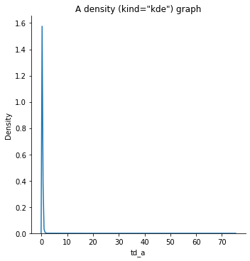
sns.displot(data=ccm,
            x='td_a',
            kind='kde').set(title='A density (kind="kde") graph')
plt.show()
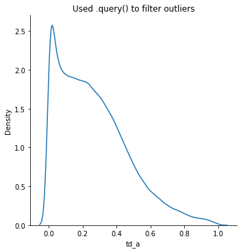
sns.displot(data=ccm.query('td_a < 1 & td_a > 0'),
            x='td_a',
            kind='kde').set(title='Used .query() to filter outliers')
plt.show()
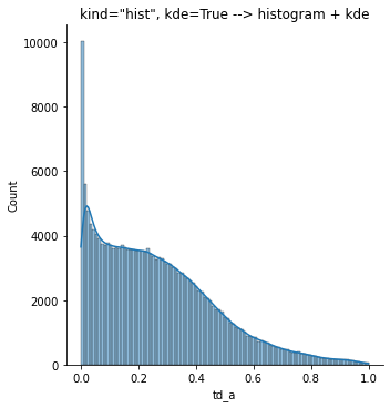
sns.displot(data=ccm.query('td_a < 1 & td_a > 0'),
            x='td_a', 
            # kind=hist is the default, so I'm not even typing it
            kde=True).set(title='kind="hist", kde=True --> histogram + kde' )
plt.show()

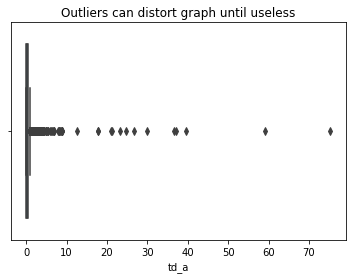
sns.boxplot(data=ccm, 
            x='td_a').set(title='Outliers can distort graph until useless')
plt.show()
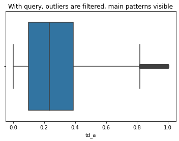
sns.boxplot(data=ccm.query('td_a < 1 & td_a > 0'), 
            x='td_a').set(title='With query, outliers are filtered, main patterns visible')
plt.show()

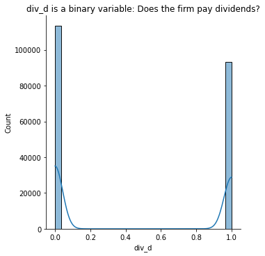
sns.displot(data = ccm,
            x = 'div_d', kde=True
           ).set(title='div_d is a binary variable: Does the firm pay dividends?')
plt.show()

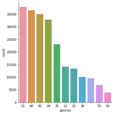
To visualize the counts of categorical variables, I’d just use pandas:

# sns.catplot is powerful, but it's overkill for a categorical count
sns.catplot(data=ccm,
            x='gsector',
            kind='count',
            order = ccm['gsector'].value_counts().index)
plt.show()

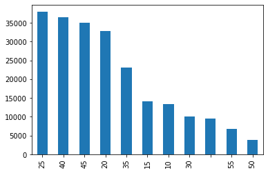
# pandas built in plot is much easier:
ccm['gsector'].value_counts().plot(kind='bar')
plt.show()

But sns.catplot is a really useful function to look at other distributional statistics for different groups!

3.3.4.4. Covariances/relationships between variables¶

To get a quick sense of relationships, I like to use I like to use pairplot and heatmap to get a quick since of relationships.

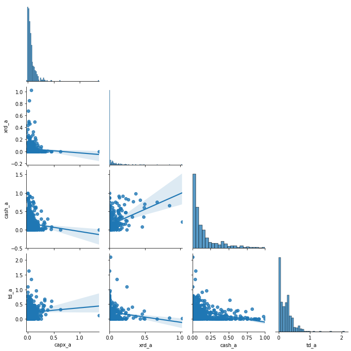
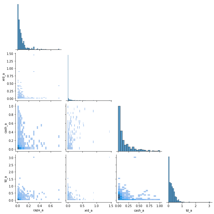
3.3.4.4.1. Getting the big picture with Pairplot¶

I like passing corner=True or using the x_vars and y_vars parameters to make the info shown more usable.

Warning

With pairplot,

Use 7 or fewer variables at a time. If your dataset has a lot of variables, do them part by part.
Don’t plot all of the data points! This will oversaturate your graphs and make it harder to draw any conclusions. Below, I randomly sample a piece of the dataset.

It’s clear from running these two plots that some extreme outliers are hiding patterns by messing with the scales and influencing the regression lines.

(We should deal with these outliers later.)

# every time you run this, you'll get diff figures... why?!
f1 = sns.pairplot(ccm[['capx_a', 'xrd_a', 'cash_a','td_a']].sample(500),
                kind='reg',
                 corner=True)
f2 = sns.pairplot(ccm[['capx_a', 'xrd_a', 'cash_a','td_a']].sample(500),
                kind='hist',
                 corner=True) # hist handles a lot of datapoints well

3.3.4.4.2. Getting the big picture with Heatmap with correlations¶

After some pairplots (and often before), I like to look at correlations.

Warning

This analysis step doesn’t help for categorical variables!

Make sure you don’t include categorical variables that are numbers!

(E.g. industry classifications are numbers that have no meaning.)

Seeing the correlations between variables is nice.

A correlation table is ugly and hard to work with:

ccm.corr()

	gvkey	fyear	lpermno	sic	sic3	age	at	me	l_a	l_sale	...	tnic3hhi	tnic3tsimm	prodmktfluid	delaycon	equitydelaycon	debtdelaycon	privdelaycon	l_emp	l_ppent	l_laborratio
gvkey	1.000000	0.534930	0.475523	0.107321	0.107265	-0.276126	0.010126	0.014763	0.126591	0.038674	...	-0.021473	0.036015	0.244347	0.212391	0.225956	-0.110047	0.276941	-0.090190	0.002419	0.103596
fyear	0.534930	1.000000	0.402615	0.098469	0.098408	0.449878	0.080264	0.142570	0.345151	0.243784	...	0.047983	-0.084418	0.060319	-0.028163	-0.037806	0.029978	-0.048051	0.029245	0.184322	0.257928
lpermno	0.475523	0.402615	1.000000	0.110724	0.110660	-0.195393	0.019407	-0.021205	0.029452	-0.042433	...	-0.019426	0.049461	0.168210	0.132109	0.150432	-0.039851	0.188820	-0.155718	-0.079054	0.054108
sic	0.107321	0.098469	0.110724	1.000000	0.999999	-0.072601	0.036937	-0.016392	0.050434	-0.031385	...	-0.052579	0.138981	0.111862	-0.034781	-0.025027	-0.067122	0.046615	-0.030025	-0.152852	-0.223692
sic3	0.107265	0.098408	0.110660	0.999999	1.000000	-0.072562	0.036988	-0.016361	0.050608	-0.031159	...	-0.052559	0.138958	0.111700	-0.034839	-0.025132	-0.066992	0.046468	-0.029792	-0.152593	-0.223594
age	-0.276126	0.449878	-0.195393	-0.072601	-0.072562	1.000000	0.079051	0.191595	0.376925	0.394578	...	0.052359	-0.154524	-0.243894	-0.210383	-0.239992	0.108078	-0.296800	0.304658	0.366293	0.187915
at	0.010126	0.080264	0.019407	0.036937	0.036988	0.079051	1.000000	0.418377	0.250631	0.192991	...	-0.034427	0.026975	0.060690	0.004913	-0.004631	0.014204	-0.031252	0.221481	0.174699	0.058018
me	0.014763	0.142570	-0.021205	-0.016392	-0.016361	0.191595	0.418377	1.000000	0.359011	0.338825	...	-0.027534	-0.029282	0.013475	-0.005837	-0.010836	-0.018789	-0.018693	0.391248	0.349469	0.142494
l_a	0.126591	0.345151	0.029452	0.050434	0.050608	0.376925	0.250631	0.359011	1.000000	0.872928	...	-0.244952	0.135873	0.070614	-0.065039	-0.139895	0.171411	-0.221926	0.718865	0.832030	0.373117
l_sale	0.038674	0.243784	-0.042433	-0.031385	-0.031159	0.394578	0.192991	0.338825	0.872928	1.000000	...	-0.108592	-0.162672	-0.164440	-0.174759	-0.276642	0.242195	-0.359774	0.805165	0.832674	0.196937
prof_a	-0.032376	-0.016935	-0.024876	0.000183	0.000213	0.036991	0.001021	0.015373	0.076535	0.111897	...	-0.006247	-0.017040	-0.048775	-0.101483	-0.144560	0.069140	-0.155657	0.057073	0.068003	0.040532
mb	0.015236	0.024092	0.018649	0.009941	0.009921	-0.008643	-0.007318	0.007431	-0.072881	-0.053002	...	0.004663	-0.017202	0.012462	0.114049	0.168112	-0.140150	0.215779	-0.038118	-0.055769	-0.052968
ppe_a	-0.135813	-0.171166	-0.127377	-0.265391	-0.265214	0.021262	-0.044536	0.014267	0.046263	0.111666	...	-0.010736	-0.274219	-0.140591	0.011186	-0.049586	0.180126	-0.179432	0.160349	0.487191	0.611810
capx_a	-0.066717	-0.163322	-0.048126	-0.128922	-0.128830	-0.126680	-0.034281	-0.014750	-0.081184	-0.062048	...	-0.025464	-0.112381	-0.014537	0.069741	0.042308	0.041066	0.000323	0.012417	0.147684	0.295649
xrd_a	0.092295	0.080038	0.064314	-0.056463	-0.056631	-0.048923	-0.019533	-0.017695	-0.180619	-0.214395	...	-0.042739	0.009194	0.169561	0.179756	0.256839	-0.156769	0.285156	-0.130468	-0.166178	-0.072052
cash_a	0.224050	0.153596	0.142805	0.039442	0.039296	-0.120339	-0.024931	-0.029058	-0.240905	-0.303408	...	-0.001263	-0.061901	0.231409	0.250270	0.356693	-0.398662	0.491385	-0.242722	-0.316222	-0.156323
div_d	-0.143810	-0.105791	-0.176155	-0.034704	-0.034589	0.209333	0.076352	0.133055	0.434820	0.411841	...	-0.097187	0.125090	-0.061720	-0.124230	-0.146363	0.095661	-0.188719	0.378149	0.409395	0.127227
td	0.003857	0.068688	0.011306	0.033958	0.033992	0.078200	0.830751	0.361632	0.224592	0.173297	...	-0.019110	0.015334	0.048355	0.013929	0.006329	0.017482	-0.017984	0.194655	0.149301	0.067114
td_a	-0.041912	-0.058602	-0.025629	-0.007453	-0.007468	0.001203	0.005640	-0.005687	0.036377	0.044912	...	-0.001006	-0.067247	-0.014955	0.013493	-0.003257	0.179656	-0.090580	0.038511	0.104232	0.156660
td_mv	-0.095096	-0.136315	-0.078023	0.058698	0.058789	0.008723	0.094805	-0.027080	0.264727	0.180944	...	-0.083947	0.224841	0.046017	-0.053045	-0.115435	0.356015	-0.276715	0.127690	0.225602	0.158872
dltt_a	-0.025243	-0.027216	-0.017234	-0.016189	-0.016199	0.034247	-0.006857	-0.004115	0.088419	0.091396	...	-0.019466	-0.093693	-0.017095	0.016273	-0.009877	0.185298	-0.099023	0.069760	0.168018	0.214947
dv_a	0.000433	0.002155	-0.006613	0.011560	0.011547	0.017824	-0.002553	0.008590	-0.002643	0.010263	...	0.020645	-0.013909	-0.015901	-0.016225	-0.023186	-0.008109	-0.027834	0.004705	0.000153	0.029392
invopps_FG09	0.014087	0.025920	0.019696	0.013651	0.013632	-0.008012	-0.009023	0.005050	-0.068388	-0.053791	...	-0.000954	0.017745	0.018953	0.119372	0.177258	-0.153368	0.230717	-0.040975	-0.057058	-0.047338
sales_g	0.002118	-0.000244	0.003401	-0.000393	-0.000395	-0.006840	-0.001200	-0.001852	-0.009331	-0.010363	...	-0.001085	-0.000550	0.009896	-0.001228	0.001472	-0.008093	0.007809	-0.008432	-0.009231	0.000193
short_debt	0.017008	-0.031044	0.031285	0.076769	0.076772	-0.112489	0.025343	-0.023332	-0.195373	-0.231229	...	0.056781	0.135594	0.030166	0.020471	0.063244	-0.129376	0.124318	-0.177918	-0.307513	-0.216896
long_debt_dum	-0.120833	-0.118462	-0.097384	-0.048407	-0.048333	0.057693	0.039313	0.054351	0.247078	0.254331	...	-0.051041	0.064945	-0.015834	-0.058475	-0.097171	0.251156	-0.196334	0.229960	0.307833	0.141860
atr	0.055605	-0.021006	0.048001	-0.057143	-0.057163	-0.130810	-0.037131	-0.076904	-0.292325	-0.280625	...	0.080345	-0.100169	0.119474	0.184233	0.242827	-0.087503	0.254502	-0.176234	-0.205942	-0.049847
smalltaxlosscarry	0.121731	0.228745	0.087134	0.011192	0.011204	0.144917	0.050115	0.090566	0.198132	0.181862	...	-0.014424	-0.055757	-0.032283	-0.042433	-0.053955	0.006375	-0.043721	0.125611	0.167890	0.094071
largetaxlosscarry	0.131454	0.176323	0.103508	-0.010460	-0.010525	-0.011025	-0.030574	-0.068973	-0.263600	-0.311908	...	0.064159	0.109787	0.180862	0.158367	0.210634	-0.070300	0.219635	-0.242570	-0.237480	0.027022
tnic3hhi	-0.021473	0.047983	-0.019426	-0.052579	-0.052559	0.052359	-0.034427	-0.027534	-0.244952	-0.108592	...	1.000000	-0.301292	-0.310163	-0.114673	-0.116476	0.051374	-0.106777	-0.053393	-0.129702	-0.132895
tnic3tsimm	0.036015	-0.084418	0.049461	0.138981	0.138958	-0.154524	0.026975	-0.029282	0.135873	-0.162672	...	-0.301292	1.000000	0.396461	0.303963	0.385465	-0.180947	0.382518	-0.165729	-0.149036	0.048841
prodmktfluid	0.244347	0.060319	0.168210	0.111862	0.111700	-0.243894	0.060690	0.013475	0.070614	-0.164440	...	-0.310163	0.396461	1.000000	0.317672	0.383794	-0.179151	0.396171	-0.192621	-0.108475	0.119382
delaycon	0.212391	-0.028163	0.132109	-0.034781	-0.034839	-0.210383	0.004913	-0.005837	-0.065039	-0.174759	...	-0.114673	0.303963	0.317672	1.000000	0.910246	-0.129176	0.530678	-0.122729	-0.067429	0.095262
equitydelaycon	0.225956	-0.037806	0.150432	-0.025027	-0.025132	-0.239992	-0.004631	-0.010836	-0.139895	-0.276642	...	-0.116476	0.385465	0.383794	0.910246	1.000000	-0.199101	0.723611	-0.184878	-0.155000	0.064953
debtdelaycon	-0.110047	0.029978	-0.039851	-0.067122	-0.066992	0.108078	0.014204	-0.018789	0.171411	0.242195	...	0.051374	-0.180947	-0.179151	-0.129176	-0.199101	1.000000	-0.490911	0.180458	0.221762	0.067969
privdelaycon	0.276941	-0.048051	0.188820	0.046615	0.046468	-0.296800	-0.031252	-0.018693	-0.221926	-0.359774	...	-0.106777	0.382518	0.396171	0.530678	0.723611	-0.490911	1.000000	-0.257807	-0.276021	-0.030851
l_emp	-0.090190	0.029245	-0.155718	-0.030025	-0.029792	0.304658	0.221481	0.391248	0.718865	0.805165	...	-0.053393	-0.165729	-0.192621	-0.122729	-0.184878	0.180458	-0.257807	1.000000	0.787591	0.028813
l_ppent	0.002419	0.184322	-0.079054	-0.152852	-0.152593	0.366293	0.174699	0.349469	0.832030	0.832674	...	-0.129702	-0.149036	-0.108475	-0.067429	-0.155000	0.221762	-0.276021	0.787591	1.000000	0.556455
l_laborratio	0.103596	0.257928	0.054108	-0.223692	-0.223594	0.187915	0.058018	0.142494	0.373117	0.196937	...	-0.132895	0.048841	0.119382	0.095262	0.064953	0.067969	-0.030851	0.028813	0.556455	1.000000

39 rows × 39 columns

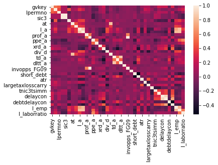
But a lazily made figure of that exact same info is somewhat workable:

f3 = sns.heatmap(ccm.corr()) # v1, use the nicer version below!

Cleaning that and making it more useful is easy:

Drop the numerical variables that don’t make sense in a correlation matrix
Make the figure large enough to see
Colors: cold for negative corr, hot for positive corr

# dont plot identifying type info or categorical vars
corr = ccm.drop(columns=['gvkey','lpermno','sic3','fyear','sic']).corr()

fig, ax = plt.subplots(figsize=(9,9)) # make a big space for the figure
ax = sns.heatmap(corr,
                 # cmap for the colors, 
                 center=0,square=True,
                 cmap=sns.diverging_palette(230, 20, as_cmap=True),
                 # mask to hide the upper diag (redundant)
                 mask=np.triu(np.ones_like(corr, dtype=bool)),
                 # shrink the heat legend
                 cbar_kws={"shrink": .5},
                 #optional: vmax and vmin will "cap" the color range
                )

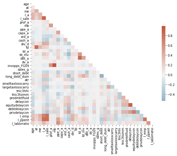
That is an information DENSE figure, but we somehow managed to get it on screen decently! Still, it’s a ton of variables, and doing this in parts would be a good idea.

Tip

If you’re feeling frisky, and your data is in good shape, you can push this farther by using sns.clustermap to find clusters of similar variables.

Also - don’t take these correlations as gospel yet: They should point you towards further relationships to explore, which you should do one plot at a time.

3.3.4.4.3. Digging in with lmplot and Jointplot¶

These are good for digging into the relationships between two continuous variables.

Let’s dig into a strong correlation suggested by our heatmap.

Warning

Jointplot can be slow - it’s doing a lot.

Again, don’t plot all of the data points! As your sample size goes up, either randomly sample data, or use “hex” style graphs.

f1 = sns.jointplot(data=ccm.query('xrd_a<.4').sample(1000),
                  x="prodmktfluid", y="xrd_a", kind='reg') 
# notice: most firms have 0 R&D!
f2 = sns.jointplot(data=ccm.query('xrd_a<.4 & xrd_a > 0').sample(1000),
                  x="prodmktfluid", y="xrd_a", kind='reg')

# set_title doesn't work with jointplots
f1.fig.suptitle('Strongly positive, even with zero R&D firms in sample')
f1.fig.subplots_adjust(top=0.95) # Reduce plot to make room 
f2.fig.suptitle('Among R&D firms, even stronger relationship')
f2.fig.subplots_adjust(top=0.95) # Reduce plot to make room 

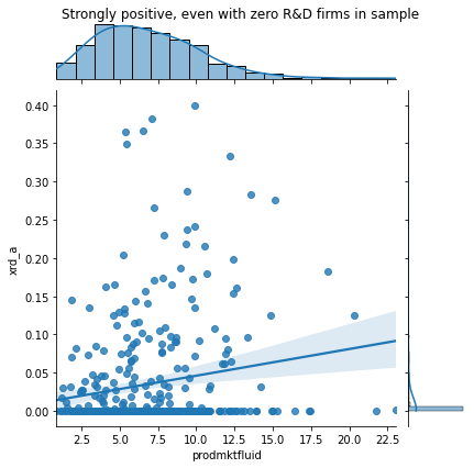
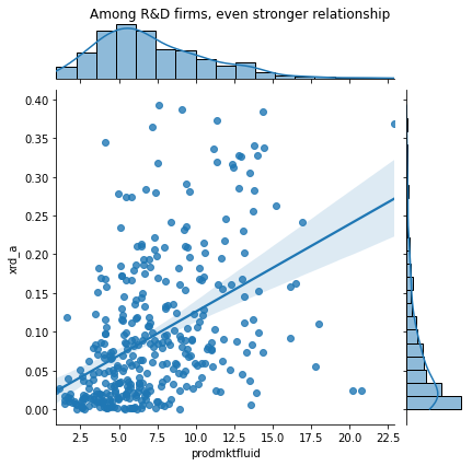
I’d pencil this as a relationship to look into more (Do firms do more R&D because of the fluidity of their product market?) and then continue exploring.

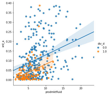
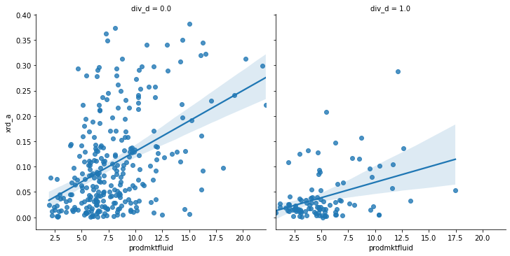
lmplot will plot regressions as well, but it makes it easy add facets to see if the relationship depends on a third (categorical) variable with the hue, col, and row parameters. (And you can combine hue, col, and row to see several cuts!)

f3 = sns.lmplot(data=ccm.query('xrd_a<.4 & xrd_a > 0').sample(1000),
                  x="prodmktfluid", y="xrd_a", hue='div_d')
f4 = sns.lmplot(data=ccm.query('xrd_a<.4 & xrd_a > 0').sample(1000),
                  x="prodmktfluid", y="xrd_a", col='div_d')

LeDataSciFi-2021

3.3.4. Visual EDA¶

3.3.4.1. EDA on a classic firm financial dataset¶

3.3.4.2. The mystery of the poorly populated variables¶

3.3.4.3. Distributions¶

3.3.4.4. Covariances/relationships between variables¶

3.3.4.4.1. Getting the big picture with Pairplot¶

3.3.4.4.2. Getting the big picture with Heatmap with correlations¶

3.3.4.4.3. Digging in with lmplot and Jointplot¶