5.4.3. Cross-Validation¶

Cross-validation is a step where we take our training sample and further divide it in many folds, as in the illustration here:

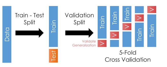
As we talked about in the last chapter, cross-validation allows us to test our models outside the training data more often. This trick reduces the likelihood of overfitting and improves generalization: It should improve our model’s performance when we apply it outside the training data.

Warning

I say “should” because the exact manner in which you create the folds matters.

Tip

This page should be your first reference for available CV splitting options.

If your data has groups (i.e. repeated observations for a given firm), you should use group-wise cross-validation, like GroupKFold to make sure no group is in the training and validation partitions of the fold.
If your data and/or task is time dependent, like predicting stock returns, you should use a time-wise cross-validation, like TimeSeriesSplit to ensure that the validation partitions are subsequent to the training sample.

5.4.3.1. Using CV in practice¶

Like before, let’s first load the data. Notice I consolidated the import lines at the top.

import pandas as pd
import numpy as np
from sklearn.linear_model import Ridge
from sklearn.model_selection import train_test_split

url        = 'https://github.com/LeDataSciFi/ledatascifi-2022/blob/main/data/Fannie_Mae_Plus_Data.gzip?raw=true'
fannie_mae = pd.read_csv(url,compression='gzip').dropna()
y          = fannie_mae.Original_Interest_Rate
fannie_mae = (fannie_mae
                  .assign(l_credscore = np.log(fannie_mae['Borrower_Credit_Score_at_Origination']),
                          l_LTV = np.log(fannie_mae['Original_LTV_(OLTV)']),
                         )
              .iloc[:,-11:] # limit to these vars for the sake of this example
             )

And, like before, we then split off some of the data into a testing sample.

For the sake of simplicity (laziness?), let’s just reuse the train_test_split approach from the last page.

rng = np.random.RandomState(0) # this helps us control the randomness so we can reproduce results exactly
X_train, X_test, y_train, y_test = train_test_split(fannie_mae, y, random_state=rng)

Back to our regularly scheduled “CV in Practice” programming.

5.4.3.2. STEP 2: Set up the CV¶

Sk-learn makes cross-validation pretty easy. We use the cross_validate("estimator",X_train,y_train,cv,scoring,...) function (documentation here) which will

Create folds in X_train and y_train using whatever method you put in the cv parameter. For each fold, it will create a smaller “training partition” and “validation partition” like in the figure at the top of this page.
For each fold,
1. It will fit your “estimator” on the smaller training partition it creates for that fold (as if you ran estimator.fit(X_trainingpartition,y_trainingpartition)).Note: Your estimator will actually be a “pipeline” object (covered in detail on the next page) that tells sk-learn to apply a series of steps to the data (preprocessing, etc.) and always ends with a model to estimate.
2. Use that fitted estimator on the validation partition (as if you ran estimator.predict(X_validationpartition)).
3. Score those predictions with the function(s) you put in scoring.
Output a dictionary object with performance data for each fold.

Important

So, to use cross_validate(), you need to decide on and set up:

Your preferred folding method (and number of folds)
Your estimator (or pipeline ending in an estimator)
Your scoring method(s)

It’s this simple:

from sklearn.model_selection import KFold, cross_validate

cv    = KFold(5)                       # set up fold method
ridge = Ridge(alpha=1.0)               # set up model/estimator
cross_validate(ridge,
               X_train,y_train, cv=cv, 
               scoring='r2')           # tell it the scoring method here

{'fit_time': array([0.01695871, 0.00604463, 0.00346589, 0.0063622 , 0.00415468]),
 'score_time': array([0.00298142, 0.0017314 , 0.00103474, 0.0025425 , 0.        ]),
 'test_score': array([0.90789446, 0.89926394, 0.900032  , 0.90479828, 0.90327986])}

Note

Wow, that was easy! Just 3 lines of code (and an import).

And we can output test score statistics like:

scores = cross_validate(ridge, X_train, y_train, cv=cv, scoring="r2")
print(scores["test_score"].mean())  # scores is just a dictionary
print(scores["test_score"].std())

0.9030537085469961
0.003162930786979486

5.4.3.3. Next step: Pipelines¶

The model above

Only uses a few continuous variables: what if we want to include other variable types (like categorical)?
Uses the variables as given: ML algorithms often need you to transform your variables
Doesn’t deal with any data problems (e.g. missing values or outliers)
Doesn’t create any interaction terms or polynomial transformations
Uses every variable I give it: But if your input data had 400 variables, you’d be in danger of overfitting!

At this point, you are capable of solving all of these problems. (For example, you could clean the data in pandas.)

But for our models to be robust to evil monsters like “data leakage”, we need the fixes to be done within pipelines.

LeDataSciFi-2022

5.4.3. Cross-Validation¶

5.4.3.1. Using CV in practice¶

5.4.3.2. STEP 2: Set up the CV¶

5.4.3.3. Next step: Pipelines¶