.ipynb .pdf

repository open issue suggest edit

Binder Colab

Contents

3.2.7. Common tasks

Important

Yes, this page is kind of long. But that’s because it has a lot of useful info!

Use the page’s table of contents to the right to jump to what you’re looking for.

3.2.7.1. Reshaping data

In the shape of data page, I explained the concept of wide vs. tall data with this example:

import pandas as pd

df = (pd.Series({   ('Ford',2000):10,
                   ('Ford',2001):12,
                   ('Ford',2002):14,
                   ('Ford',2003):16,
                   ('GM',2000):11,
                   ('GM',2001):13,
                   ('GM',2002):13,
                   ('GM',2003):15})
      .to_frame()
      .rename(columns={0:'Sales'})
      .rename_axis(['Firm','Year'])
      .reset_index()
     )
print("Tall:")
display(df)

Tall:

	Firm	Year	Sales
0	Ford	2000	10
1	Ford	2001	12
2	Ford	2002	14
3	Ford	2003	16
4	GM	2000	11
5	GM	2001	13
6	GM	2002	13
7	GM	2003	15

Note

To reshape dataframes, you have to work with index and column names.

So before we use stack and unstack here, put the firm and year into the index.

tall = df.set_index(['Firm','Year'])

3.2.7.1.1. To convert a tall dataframe to wide: df.unstack().

If your index has multiple levels, the level parameter is used to pick which to unstack. “0” is the innermost level of the index.

print("\n\nUnstack (make it shorter+wider) on level 0/Firm:\n") 
display(tall.unstack(level=0))
print("\n\nUnstack (make it shorter+wider) on level 1/Year:\n") 
display(tall.unstack(level=1))

Unstack (make it shorter+wider) on level 0/Firm:

	Sales
Firm	Ford	GM
Year
2000	10	11
2001	12	13
2002	14	13
2003	16	15

Unstack (make it shorter+wider) on level 1/Year:

	Sales
Year	2000	2001	2002	2003
Firm
Ford	10	12	14	16
GM	11	13	13	15

3.2.7.1.2. To convert a wide dataframe to tall/long: df.stack().

Tip

Pay attention after reshaping to the order of your index variables and how they are sorted.

# save the wide df above to this name for subseq examples
wide_year = tall.unstack(level=0) 

print("\n\nStack it back (make it tall): wide_year.stack()\n") 
display(wide_year.stack())
print("\n\nYear-then-firm doesn't make much sense.\nReorder to firm-year: wide_year.stack().swaplevel()") 
display(wide_year.stack().swaplevel())
print("\n\nYear-then-firm sorting make much sense.\nSort to firm-year: wide_year.stack().swaplevel().sort_index()") 
display(wide_year.stack().swaplevel().sort_index())

Stack it back (make it tall): wide_year.stack()

		Sales
Year	Firm
2000	Ford	10
	GM	11
2001	Ford	12
	GM	13
2002	Ford	14
	GM	13
2003	Ford	16
	GM	15

Year-then-firm doesn't make much sense.
Reorder to firm-year: wide_year.stack().swaplevel()

		Sales
Firm	Year
Ford	2000	10
GM	2000	11
Ford	2001	12
GM	2001	13
Ford	2002	14
GM	2002	13
Ford	2003	16
GM	2003	15

Year-then-firm sorting make much sense.
Sort to firm-year: wide_year.stack().swaplevel().sort_index()

		Sales
Firm	Year
Ford	2000	10
	2001	12
	2002	14
	2003	16
GM	2000	11
	2001	13
	2002	13
	2003	15

Beautiful!

3.2.7.2. Lambda (in assign or after groupby)

You will see this inside pandas chains a lot: lambda x: someFunc(x), e.g.:

• .assign(lev = lambda x: (x['dltt']+x['dlc'])/x['at']  )

• .groupby('industry').assign(avglev = lambda x: x['lev'].mean()  )

Q1: What is that “lambda”?

A1: A lambda function is an anonymous function that is usually one line and usually defined without a name. You write it like this:

lambda <list the input(s)>: <expression that uses the inputs to make an output>

Here, you can see how the lambda function takes inputs and creates output the same way a function does:

dumb_prog = lambda a: a + 10     # I added "dumb_prog =" to name the lambda function and use it
dumb_prog(5)

15

# we could define a fnc to do the exact same thing
def dumb_prog(a):
    return a + 10
dumb_prog(5)

15

Q2: Why is that lambda there?

A2: We use lambdas when we need a function for a short period of time and when the name of the function doesn’t matter.

In the example above, [df].groupby('industry').assign(avglev = lambda x: x['lev'].mean()  ),

1. groupby splits the dataframe into groups,

2. then, within each group, it applies a function (here: the mean),

3. and then returns a new dataframe with one observation for each group (the average leverage for the industry). Visually, this split-apply-combine1 process looks like this:

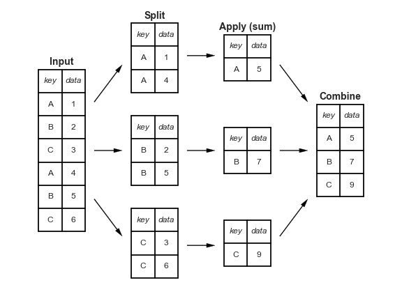
But notice! The .assign() portion is working on these tiny split up pieces of the dataframe created by df.groupby('industry'). Those pieces are dataframe objects that don’t have names!

So lambda functions let us refer to an unnamed dataframe objects! When you type <some df object, like df.groupby()>.assign(newVar = lambda x: someFunc(x)), x is the object (“some df object”) that assign is working on. Ta da!

# common syntax within pandas
.assign(<newvarname> = lambda <tempnameforpriorobj>:  <do stuff to tempnameforpriorobj>   )       

# often, tempname is just "x" for short
.assign(<newvarname> = lambda x: <someFunc(x)> )      

# example:
.assign(lev = lambda x: (x['dltt']+x['dlc'])/x['at'] )

Note

It turns out that lambda functions are very useful in python programming, and not just within pandas. For example, some functions take functions as inputs, like csnap(), map(), and filter(), and lambda functions lets us give them custom functions quickly.

But pandas is where we will use lambda functions most in this class.

3.2.7.3. .transform() after groupby

Sometimes you get a statistic for a group, but you want that statistic in every single row of your original dataset.

But groupby creates a new dataframe that is smaller, with only one row per row.

import pandas as pd 
import numpy as np
df = pd.DataFrame({'key':["A",'B','C',"A",'B','C'],
                   'data':np.arange(1,7)}).set_index('key').sort_index()

display(df) # the input

	data
key
A	1
A	4
B	2
B	5
C	3
C	6

# groupby().sum() shrinks the dataset
display(df.groupby(level='key')['data'].sum()
       .to_frame() ) # just added this line bc df prints prettier than series

	data
key
A	5
B	7
C	9

# groupby().transform(sum) does NOT shrink the dataset

df.groupby(level='key').transform(sum)    

	data
key
A	5
A	5
B	7
B	7
C	9
C	9

One last trick: Let’s add that new variable to the original dataset!

# option 1: create the var
df['groupsum'] = df.groupby(level='key').transform(sum)

# option 2: create the var with assign (can be used inside chains)
df = df.assign(groupsum = df.groupby(level='key')['data'].transform(sum))

display(df) 

	data	groupsum
key
A	1	5
A	4	5
B	2	7
B	5	7
C	3	9
C	6	9

3.2.7.4. Using non-pandas functions inside chains

One problem with writing chains on dataframes is that you can only use methods that work on the object (a dataframe) that is getting chained.

So for example, you’ve formatted dataframe to plot. You can’t directly add a seaborn function to the chain: Seaborn functions are methods of the package seaborn, not the dataframe. (It’s sns.lmplot, not df.lmplot.)

.pipe() allows you to hand a dataframe to functions that don’t work directly on dataframes.

The syntax of .pipe()

df.pipe(<'outside function'>, 
        <'if the first parameter of the outside function isnt the df, '
         'the name of the parameter that is expecting the dataframe'>,
        <'any other parameters youd give the outside function'>

Note that the object after the pipe command is run might not be a dataframe anymore! It’s whatever object the piped function produces!

3.2.7.4.1. Example 1

From one of the pandas devs:

jack_jill = pd.DataFrame()
(jack_jill.pipe(went_up, 'hill')
    .pipe(fetch, 'water')
    .pipe(fell_down, 'jack')
    .pipe(broke, 'crown')
    .pipe(tumble_after, 'jill')
)

This really is just right-to-left function execution. The first argument to pipe, a callable, is called with the DataFrame on the left as its first argument, and any additional arguments you specify.

I hope the analogy to data analysis code is clear. Code is read more often than it is written. When you or your coworkers or research partners have to go back in two months to update your script, having the story of raw data to results be told as clearly as possible will save you time.

3.2.7.4.2. Example 2

From Steven Morse:

(sns.load_dataset('diamonds')
 .query('cut in ["Ideal", "Good"] & \
         clarity in ["IF", "SI2"] & \
         carat < 3')
 .pipe((sns.FacetGrid, 'data'),
        row='cut', col='clarity', hue='color',
        hue_order=list('DEFGHIJ'),
        height=6,
        legend_out=True)
 .map(sns.scatterplot, 'carat', 'price', alpha=0.8)
 .add_legend())

3.2.7.5. Printing inside of chains

Tip

One thing about chains, is that sometimes it’s hard to know what’s going on within them without just commenting out all the code and running it bit-by-bit.

This function, csnap (meaning “C”hain “SNAP”shot) will let you print messages from inside the chain, by exploiting the .pipe() function we just covered!

Copy this into your code:

def csnap(df, fn=lambda x: x.shape, msg=None):
    """ Custom Help function to print things in method chaining.    
        Will also print a message, which helps if you're printing a bunch of these, so that you know which csnap print happens at which point.
        Returns back the df to further use in chaining.
        
        Usage examples - within a chain of methods:
            df.pipe(csnap)
            df.pipe(csnap, lambda x: <do stuff>)
            df.pipe(csnap, msg="Shape here")
            df.pipe(csnap, lambda x: x.sample(10), msg="10 random obs")
    """
    if msg:
        print(msg)
    display(fn(df))
    return df

An example of this in use:

(df
 .pipe(csnap, msg="Shape before describe")
 .describe()['data']  # get the distribution stats of a variable (I'm just doing something to show csnap off)
 .pipe(csnap, msg="Shape after describe and pick one var") # see, it prints a message from within the chain!
 .to_frame()
 .assign(ones = 1)
 .pipe(csnap, lambda x: x.sample(2), msg="Random sample of df at point #3") # see, it prints a message from within the chain! 
 .assign(twos=2,threes=3)
)

Shape before describe

(6, 2)

Shape after describe and pick one var

(8,)

Random sample of df at point #3

	data	ones
max	6.0	1
min	1.0	1

	data	ones	twos	threes
count	6.000000	1	2	3
mean	3.500000	1	2	3
std	1.870829	1	2	3
min	1.000000	1	2	3
25%	2.250000	1	2	3
50%	3.500000	1	2	3
75%	4.750000	1	2	3
max	6.000000	1	2	3

3.2.7.6. Prettier pandas output

A few random things:

• Want to change the order of rows in an output table? .reindex()

• Want to format the numbers shown by pandas?

  1. Permanent: Add this line of code to the top of your file: pd.set_option('display.float', '{:.2f}'.format)

  2. Temp:Add style.format to the end of your table command. E.g.: df.describe().style.format("{:.2f}")

• Want to control the number of columns / rows pandas shows?

  1. pd.set_option('display.max_columns', 50)

  2. pd.set_option('display.max_rows', 50)

• More formatting controls: https://pandas.pydata.org/pandas-docs/stable/reference/api/pandas.set_option.html

---

1

(This figure is yet another resource I’m borrowing from the awesome PythonDataScienceHandbook.

3.2.6. Using “method chains” to create more readable code 3.2.8. Exercises