9.6. Is signal X useful in predicting returns?¶

In many “cross-sectional” asset pricing papers, the main results are shown in Table 1, and show whether we can form portfolios that generate alpha using some signal (a variable that describes something about stocks) to sort stocks into portfolios.

To make this analysis more rigorous, we can measure alpha six different ways (against six different asset pricing models). Among these are the CAPM and FF3 models we just estimated in prior pages.

The basic idea of this kind of table is that

We measure something about stocks. Maybe it’s their size, or their recent returns. Let’s call this variable X.
Then we sort stocks on X every month and divide them into 5 or 10 buckets. The stocks in each bucket constitute a portfolio, so we get the returns for that bucket for the next month. We also compute the “Long-Short” portfolio, which is always the return of the highest bucket minus the lowest bucket. The long-short portfolio is what you would get if you short the stocks in the lowest bucket to go long the highest bucket, and are “zero cost” portfolios.
We repeat this across time so we can see how each portfolio/bucket does and show the average return in each bucket.
To be more sophisticated, we do step 3 a few ways: We look at the portfolio returns compared to the market, and we also compute the portfolio alphas against some benchmark factor models.
If we see significant results in the High Minus Low column, practitioners will say that X is an “anomaly”, in that the asset pricing model can’t explain its returns.

The plan for this code file comes from the “Assaying Anomalies” project, which is a protocol to evaluate whether a given factor X is useful in predicting returns.

Here is the repo containing that project’s code (mostly in Matlab as of Spring 2025, but will be in Python soon).
The paper describing that project, which you should read (it is breezy), and what you should cite is: Novy-Marx, Robert and Velikov, Mihail, Assaying Anomalies (February 13, 2024). Available at SSRN: https://ssrn.com/abstract=4338007 or http://dx.doi.org/10.2139/ssrn.4338007
If you want to go beyond the Table 1 we output here, the next things you should output are precisely what Velikov and Novy-Marx show in their paper after Table 1.

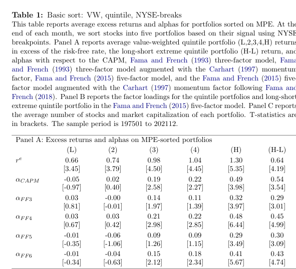
9.6.1. What “Table 1” looks like¶

In our code below, we are trying to replicate the structure of this table below, from Novy-Marx and Velikov.

# !pip install pandas-datareader # run this once, then comment

import pandas_datareader.famafrench as ff
import pandas as pd
import numpy as np
import statsmodels.api as sm
import statsmodels.formula.api as smf
import warnings
warnings.simplefilter(action="ignore", category=FutureWarning)

# datasets = ff.get_available_datasets()
# datasets

9.6.2. Step 1: Get the factor portfolio returns.¶

df_factors = ff.FamaFrenchReader('F-F_Research_Data_5_Factors_2x3', start='1900-01-01').read()[0]

# add momentum to this
mom = ff.FamaFrenchReader('F-F_Momentum_Factor', start='1900-01-01').read()[0] # add momentum
mom.columns = ['Mom'] # rename
df_factors = pd.merge(df_factors, mom, left_index=True, right_index=True)
df_factors # FYI: contains Mkt-RF and RF, but no Mkt

	Mkt-RF	SMB	HML	RMW	CMA	RF	Mom
Date
1963-07	-0.39	-0.41	-0.97	0.68	-1.18	0.27	0.90
1963-08	5.07	-0.80	1.80	0.36	-0.35	0.25	1.01
1963-09	-1.57	-0.52	0.13	-0.71	0.29	0.27	0.19
1963-10	2.53	-1.39	-0.10	2.80	-2.01	0.29	3.12
1963-11	-0.85	-0.88	1.75	-0.51	2.24	0.27	-0.74
...	...	...	...	...	...	...	...
2024-08	1.61	-3.65	-1.13	0.85	0.86	0.48	4.79
2024-09	1.74	-1.02	-2.59	0.04	-0.26	0.40	-0.60
2024-10	-0.97	-0.88	0.89	-1.38	1.03	0.39	2.87
2024-11	6.51	4.78	-0.05	-2.62	-2.17	0.40	0.90
2024-12	-3.17	-3.87	-2.95	1.82	-1.10	0.37	0.05

738 rows × 7 columns

9.6.3. Step 2: Construct portfolio returns from your signal¶

Above, we said that

We measure something about stocks. Maybe it’s their size, or their recent returns. Let’s call this variable X.

Then we sort stocks on X every month and divide them into 5 or 10 buckets. The stocks in each bucket constitute a portfolio, so we get the returns for that bucket for the next month. We also compute the “Long-Short” portfolio, which is always the return of the highest bucket minus the lowest bucket. The long-short portfolio is what you would get if you short the stocks in the lowest bucket to go long the highest bucket, and are “zero cost” portfolios.

This is where you would do that.

For simplicity, I’m just using pre-constructed portfolio returns on this page. To see one way to construct a signal from predictor variables and how we calculate the portfolio returns, visit the page on trading on stock return predictions.

# now, here we'd develop some "signal" and then create portfolio rets based on it
# I'm skipping... you figure that out

# I'll pretend I did that by grabbing 5 industry portfolio returns
df_portfolios = ff.FamaFrenchReader('5_Industry_Portfolios', start='1900-01-01').read()[0]
df_portfolios.columns = [f'Port{i+1}' for i in range(len(df_portfolios.columns))] # this is my anticipated portfolio number name scheme

df_portfolios.eval("HmL = Port5-Port1", inplace=True)

# Make each portfolio (except for HmL) excess returns
for col in ['Port1', 'Port2', 'Port3', 'Port4', 'Port5']:
    df_portfolios[col] = df_portfolios[col] - df_factors['RF']

portfolios = df_portfolios.columns.tolist()

df_portfolios

9.6.4. Step 3: Run the regressions.¶

reg_df = pd.merge(df_factors, df_portfolios, left_index=True, right_index=True)
reg_df

	Mkt-RF	SMB	HML	RMW	CMA	RF	Mom	Port1	Port2	Port3	Port4	Port5	HmL
Date
1975-01	13.66	12.91	8.28	-0.78	-0.90	0.58	-13.82	21.19	11.94	12.90	-1.32	17.31	-3.88
1975-02	5.56	-0.65	-4.45	1.16	-2.11	0.43	-0.61	4.23	4.63	9.34	15.61	2.44	-1.79
1975-03	2.66	4.00	2.38	1.26	-1.33	0.41	-2.04	7.75	1.40	-0.17	0.88	3.74	-4.01
1975-04	4.23	-0.71	-1.14	1.41	-1.34	0.44	1.38	2.75	6.82	2.53	0.21	2.83	0.08
1975-05	5.19	2.89	-4.10	-0.98	-0.60	0.44	-0.58	3.60	5.95	4.56	6.08	5.28	1.68
...	...	...	...	...	...	...	...	...	...	...	...	...	...
2024-08	1.61	-3.65	-1.13	0.85	0.86	0.48	4.79	0.57	0.70	0.86	5.96	2.55	1.98
2024-09	1.74	-1.02	-2.59	0.04	-0.26	0.40	-0.60	4.01	1.54	2.69	-2.21	0.26	-3.75
2024-10	-0.97	-0.88	0.89	-1.38	1.03	0.39	2.87	-2.08	-2.38	-0.48	-3.50	0.72	2.80
2024-11	6.51	4.78	-0.05	-2.62	-2.17	0.40	0.90	10.52	6.01	4.76	-0.98	9.83	-0.69
2024-12	-3.17	-3.87	-2.95	1.82	-1.10	0.37	0.05	-0.82	-8.38	0.56	-5.79	-7.46	-6.64

600 rows × 13 columns

# define factor model formulas (these are the right side of the regression formulas)
# these are how formulas are specified for statsmodel's formula api
factor_models = {
    'r^e':  '1',
    'CAPM': 'Q("Mkt-RF")',
    'FF3':  'Q("Mkt-RF") + SMB + HML',
    'FF4':  'Q("Mkt-RF") + SMB + HML + Mom',
    'FF5':  'Q("Mkt-RF") + SMB + HML + RMW + CMA',
    'FF6':  'Q("Mkt-RF") + SMB + HML + RMW + CMA + Mom'
}

# pre built output table

index = pd.MultiIndex.from_product([factor_models.keys(), ['alpha', 't-stat']], names=['Model', 'Metric'])
results = pd.DataFrame(index=index, columns=portfolios, dtype=float)
results

		Port1	Port2	Port3	Port4	Port5	HmL
Model	Metric
r^e	alpha	NaN	NaN	NaN	NaN	NaN	NaN
r^e	t-stat	NaN	NaN	NaN	NaN	NaN	NaN
CAPM	alpha	NaN	NaN	NaN	NaN	NaN	NaN
CAPM	t-stat	NaN	NaN	NaN	NaN	NaN	NaN
FF3	alpha	NaN	NaN	NaN	NaN	NaN	NaN
FF3	t-stat	NaN	NaN	NaN	NaN	NaN	NaN
FF4	alpha	NaN	NaN	NaN	NaN	NaN	NaN
FF4	t-stat	NaN	NaN	NaN	NaN	NaN	NaN
FF5	alpha	NaN	NaN	NaN	NaN	NaN	NaN
FF5	t-stat	NaN	NaN	NaN	NaN	NaN	NaN
FF6	alpha	NaN	NaN	NaN	NaN	NaN	NaN
FF6	t-stat	NaN	NaN	NaN	NaN	NaN	NaN

# Run regressions for each portfolio and model

full_reg_output = {} # to save everything, in case we want to access other stuff (like beta loadings)
for portfolio in portfolios:
    for model_name, formula in factor_models.items():
        reg = smf.ols(formula=f'{portfolio} ~ {formula}', data=reg_df).fit()
        # extract the intercept coef and t-stat
        alpha = reg.params['Intercept']
        t_stat = reg.tvalues['Intercept']
        results.at[(model_name, 'alpha'), portfolio] = alpha
        results.at[(model_name, 't-stat'), portfolio] = t_stat
        full_reg_output[(model_name, portfolio)] = reg

results

		Port1	Port2	Port3	Port4	Port5	HmL
Model	Metric
r^e	alpha	0.661057	0.557900	0.646938	0.681369	0.597724	-0.063333
r^e	t-stat	3.900987	3.433497	3.230902	3.859817	3.052126	-0.647961
CAPM	alpha	0.114768	0.038745	0.010464	0.203102	-0.043658	-0.158426
CAPM	t-stat	1.630695	0.550711	0.118044	1.773375	-0.584753	-1.670608
FF3	alpha	0.091171	-0.052544	0.137807	0.302106	-0.186326	-0.277498
FF3	t-stat	1.290888	-0.815539	1.721098	2.730282	-3.023698	-3.132967
FF4	alpha	0.124516	-0.093283	0.208553	0.235236	-0.152898	-0.277413
FF4	t-stat	1.733414	-1.427806	2.585315	2.095277	-2.442501	-3.067951
FF5	alpha	-0.074883	-0.184758	0.318594	0.133618	-0.180963	-0.106080
FF5	t-stat	-1.142738	-2.948850	4.167975	1.209001	-2.945735	-1.222041
FF6	alpha	-0.032642	-0.206952	0.362788	0.093130	-0.155887	-0.123244
FF6	t-stat	-0.496089	-3.265914	4.717103	0.833356	-2.511528	-1.400810

LeDataSciFi-2025

9.6. Is signal X useful in predicting returns?¶

9.6.1. What “Table 1” looks like¶

9.6.2. Step 1: Get the factor portfolio returns.¶

9.6.3. Step 2: Construct portfolio returns from your signal¶

9.6.4. Step 3: Run the regressions.¶