9.3. Expanding returns¶

9.3.1. The problem¶

You know the charts that show cumulative returns if you’d bought and held a stock since some long ago date? Let’s make one!

This is called “expanding returns” because you get the total returns from day 0 to day N, then from day 0 to day N+1, and so on; the window is expanding instead of having a fixed number of units or containing a specific increment of time.

9.3.2. Download the returns¶

We need a dataset with firm, date, and the daily return. Let’s build it:

#!pip install pandas_datareader # uncomment and run this ONE TIME ONLY to install pandas data reader

import pandas as pd
import numpy as np
import pandas_datareader as pdr # you might need to install this (see above)
from datetime import datetime
import yfinance as yf

# choose your firms and dates 
stocks = ['SBUX','AAPL','MSFT']
start  = datetime(1980, 1, 1)
end    = datetime(2022, 7, 31)

Tip

The code in the next block is explained more thoroughly in handouts/factor_loading_simple.ipynb in the textbook repo because that file prints the status of the data throughout. Looking at this might help.

# download stock prices 
# here, from yahoo: not my fav source, but quick. 
# we need to do some data manipulation to get the data ready 
stock_prices         = yf.download(stocks, start , end)
stock_prices.index   = stock_prices.index.tz_localize(None)      # change yf date format to match pdr
stock_prices         = stock_prices.filter(like='Adj Close')     # reduce to just columns with this in the name
stock_prices.columns = stock_prices.columns.get_level_values(1)  # tickers as col names, works no matter order of tics

# refmt from wide to long
stock_prices = stock_prices.stack().swaplevel().sort_index().reset_index()
stock_prices.columns = ['Firm','Date','Adj Close']

# add return var = pct_change() function compares to prior row
# EXCEPT: don't compare for first row of one firm with last row of prior firm!
# MAKE SURE YOU CREATE THE VARIABLES WITHIN EACH FIRM - use groupby
stock_prices['ret'] = stock_prices.groupby('Firm')['Adj Close'].pct_change()
stock_prices['ret'] = stock_prices['ret'] 
stock_prices.head(15)

	Firm	Date	Adj Close	ret
0	AAPL	1980-12-12	0.100040	NaN
1	AAPL	1980-12-15	0.094820	-0.052171
2	AAPL	1980-12-16	0.087861	-0.073398
3	AAPL	1980-12-17	0.090035	0.024751
4	AAPL	1980-12-18	0.092646	0.028992
5	AAPL	1980-12-19	0.098300	0.061029
6	AAPL	1980-12-22	0.103084	0.048670
7	AAPL	1980-12-23	0.107434	0.042199
8	AAPL	1980-12-24	0.113088	0.052628
9	AAPL	1980-12-26	0.123527	0.092310
10	AAPL	1980-12-29	0.125267	0.014083
11	AAPL	1980-12-30	0.122222	-0.024304
12	AAPL	1980-12-31	0.118743	-0.028468
13	AAPL	1981-01-02	0.120048	0.010988
14	AAPL	1981-01-05	0.117438	-0.021738

9.3.3. Getting the expanding returns¶

Notice that this dataset has the simple return for a period, not the gross returns (defined here).

To compute \(R_i[0,T]\) for all firms \(i\) and each time \(T\) in the dataset, you’re going to need to use groupby. You have two equivalent options from there:

For each firm, get the cumprod() of the gross return over its time series.
```
df.assign(R=1+df['r']).groupby('firm')['R'].cumprod()
```
For each firm, take the product of \(1+r\) for all prior periods using the expanding window functionality.
```
df.groupby('firm')['r'].expanding().apply(lambda x: np.prod(1+x))
```

Which you choose is up to you, but in my testing, the cumprod approach is 2.5x faster.

stock_prices['cumret'] = \
(
    stock_prices
    .assign(ret=1+stock_prices['ret'])
    .groupby('Firm')
    ['ret']
    .cumprod()
)

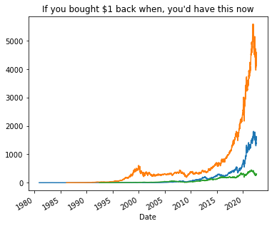
9.3.4. Plotting the total returns¶

If only we could turn back time.

(stock_prices.set_index('Date').groupby('Firm')['cumret']
 .plot(title="If you bought $1 back when, you'd have this now",
       figsize=(6,5))
);

LeDataSciFi-2025